Category: Uncategorized

Welcome to my number fifteen in my series of WebGL tutorials! In it, we’ll take a look specular maps, which give your scenes greater realism by making it easy to specify how reflective an object is at every point on its surface, just as normal textures allow you to specify its detailed colour. In terms of new code, this is actually a pretty simple extension on top of what we’ve already covered, but conceptually it’s a bit of a jump.

Here’s what the lesson looks like when run on a browser that supports WebGL:

Click here and you’ll see the live WebGL version, if you’ve got a browser that supports it; here’s how to get one if you don’t. You’ll see a spinning model of the Earth, with a very bright specular glint — the reflection of the Sun from its surface. More importantly, if you look closely, you’ll see that the specular glint only appears on the oceans; the land, as you’d expect, doesn’t reflect the light in a specular fashion.

Try switching off the “Use specular map” toggle underneath the canvas. You’ll see that now the specular highlight appears on the land too; you might also feel (as I did) that this rather ruins the illusion, and makes the specular glint look more like a very bright spotlight being shone at the Earth. Specular maps can really improve realism by giving you fine-grained control over the way objects in your model interact with the lighting.

Next, switch the “Use specular map” back on, reduce the diffuse light’s intensity to, say, (0.5, 0.5, 0.5), and then switch off the “Use color map” toggle. You’ll see that the colour texture of the earth is lost, but the specular highlight is still affected by whether or not it would be over land or sea.

So, how does it work? Read on to find out.

Before we wade into the code, the usual warning: these lessons are targeted at people with a reasonable amount of programming knowledge, but no real experience in 3D graphics; the aim is to get you up and running, with a good understanding of what’s going on, so that you can start producing your own 3D Web pages as quickly as possible. If you haven’t read the previous tutorials already, you should probably do so before reading this one — here I will only explain the new stuff. The lesson is based on lesson 14, so you should make sure that you understand that one.

There may be bugs and misconceptions in this tutorial. If you spot anything wrong, let me know in the comments and I’ll correct it ASAP.

There are two ways you can get the code for this example; just “View Source” while you’re looking at the live version, or if you use GitHub, you can clone it (and the other lessons) from the repository there.

Before we take a look at the code, it’s probably worth explaining the background. So far, we’ve been treating textures as a nice easy way of “skinning” our 3D objects with images. We specify an image, and our object has per-vertex coordinates to say which part of the image should go where, so when we draw each pixel in the object in our fragment shader, we can work out the portion of the image that corresponds to that part of the object, take its colour from the sampler object that represents the texture in the shader, and use that as the colour of the object at that point.

Specular maps take this logic one step further. The colour of a point in the texture is, of course, specified by red, green, blue, and alpha components. In the shader, each of these is a floating point number. But there’s no particular reason why we have to use them as colour values. You will remember from the last lesson that the shininess of a material is determined by a single floating point number. There’s no reason why we shouldn’t use textures as a way of passing a “shininess map” up to the fragment shader, just as we normally use it to pass a colour map.

So that’s the trick we use in this example. Two separate textures are passed up to the fragment shader to use on the Earth; a colour map that looks like this:

…and a lower-resolution specular map, which looks like this:

This is just a regular GIF file, which I created in Paint.NET using the colour map as a starting point. I decided to set the red, green and blue components of the colour at each point to the same value: the shininess of the point. I also needed to choose a value that would mean “this bit of the Earth is not shiny”; because most of the image was pretty dark (a shininess of 32 leads to the RGB colour of 32, 32, 32, which is a very dark grey) I decide to use pure white for that.

So, with all that explained, let’s go to the code. The differences between the code for this lesson and lesson 14’s are actually quite minimal, and pretty clear. As you might expect, the really important stuff is in the fragment shader, so let’s take a look at that (with changed stuff highlighted in red, as usual).

The first change is that we have a couple of new uniforms specifying whether or not we want to use the colour and specular maps:

  precision mediump float;

  varying vec2 vTextureCoord;
  varying vec3 vTransformedNormal;
  varying vec4 vPosition;

  uniform bool uUseColorMap;
  uniform bool uUseSpecularMap;
  uniform bool uUseLighting;

Next, we have uniform samplers for the two textures. We’ve renamed the old uSampler, which was used for the colour texture, to uColorMapSampler, and added a new one for the sampler that represents the specular map.

  uniform vec3 uAmbientColor;

  uniform vec3 uPointLightingLocation;
  uniform vec3 uPointLightingSpecularColor;
  uniform vec3 uPointLightingDiffuseColor;

  uniform sampler2D uColorMapSampler;
  uniform sampler2D uSpecularMapSampler;

Next comes our normal boilerplate code to handle the case where the user wants to switch off lighting effects, and to calculate the normal and the light direction if they don’t:

  void main(void) {
    vec3 lightWeighting;
    if (!uUseLighting) {
      lightWeighting = vec3(1.0, 1.0, 1.0);
    } else {
      vec3 lightDirection = normalize(uPointLightingLocation - vPosition.xyz);
      vec3 normal = normalize(vTransformedNormal);

And finally we get the code that actually handles the specular map. Firstly, we define a variable that will hold the amount of specular lighting we’re going to apply; this will, of course, be zero if the fragment we’re considering turns out to have no specular lighting after we’ve done all the calculations.

      float specularLightWeighting = 0.0;

Next, we want to work out the shininess for this bit of the material. If the user has specified that we shouldn’t use the specular map, this code makes the (essentially arbitrary) choice of using 32.0. Otherwise, we get the value from the specular map’s value for the fragment’s texture coordinates, just as we would previously have found the colour maps’ value. Now, our specular map actually has the shininess value stored in all three components of the colour at each image — red, green and blue are all the same, which is why it appears as greyscale when viewed as an image. We use the red one in this code, though we could have used either of the others if we’d wanted to:

      float shininess = 32.0;
      if (uUseSpecularMap) {
        shininess = texture2D(uSpecularMapSampler, vec2(vTextureCoord.s, vTextureCoord.t)).r * 255.0;
      }

Now, you’ll remember that we needed some way of saying “this bit of the material is not shiny” in the specular map, and that I chose to use white, as that had good contrast against the dark-grey areas for the shinier parts of the Earth. So we don’t do any calculations for specular lighting if the value for the shininess as extracted from the map is greater than or equal to 255.

      if (shininess < 255.0) {

The next bit of code is just the same specular highlight calculation we had in the last lesson, except that we use the shininess constant that we extracted from the map:

        vec3 eyeDirection = normalize(-vPosition.xyz);
        vec3 reflectionDirection = reflect(-lightDirection, normal);

        specularLightWeighting = pow(max(dot(reflectionDirection, eyeDirection), 0.0), shininess);
      }

And finally, we add all of the different forms of lighting’s contributions together, and use that to weight the colour of the fragment, whether it’s from the colour map or, if uUseColorMap is false, just a constant white.

      float diffuseLightWeighting = max(dot(normal, lightDirection), 0.0);
      lightWeighting = uAmbientColor
        + uPointLightingSpecularColor * specularLightWeighting
        + uPointLightingDiffuseColor * diffuseLightWeighting;
    }

    vec4 fragmentColor;
    if (uUseColorMap) {
      fragmentColor = texture2D(uColorMapSampler, vec2(vTextureCoord.s, vTextureCoord.t));
    } else {
      fragmentColor = vec4(1.0, 1.0, 1.0, 1.0);
    }
    gl_FragColor = vec4(fragmentColor.rgb * lightWeighting, fragmentColor.a);
  }

If you’ve got this far, you actually understand everything there is to know about the code for this lesson. There are other changes, but none are worth a detailed code walkthrough. initShaders has new code to deal with the new uniforms, initTextures needs to load the two new textures, the code that loaded up the teapot is replaced by an initBuffers function just like the one from lesson 11, drawScene has code to draw a sphere rather than a teapot, and to take the values in the user-input fields below the canvas and put them into the appropriate uniforms, and animate has been updated to make the earth spin.

And after that, that’s it! You now know how to use a texture to provide information about an object’s specular shininess. As you’ve no doubt worked out by this point, there’s nothing to stop you from using textures to pass up other fine-grained information to your shaders — people often use similar techniques to this for giving detailed maps of the variations in the surface normals, which allows you to have subtly bumpy surfaces without having to create lots of vertices. We’ll take a closer look at that in a future lesson.

<< Lesson 14Lesson 16 >>

Acknowledgments: the Earth texture is courtesy of the European Space Agency/Envisat. Thanks also to Paul Brunt for his suggestion to increase the specular lighting levels to make the demo page for this lesson clearer.

Welcome to my number thirteen in my series of WebGL tutorials! In it, we’ll cover per-fragment lighting, which is harder work for the graphics card than the per-vertex lighting we’ve been doing so far, but gives much more realistic results. We’ll also look at how you can switch the shaders used by your code by changing which WebGL program object is in use.

Here’s what the lesson looks like when run on a browser that supports WebGL:

Click here and you’ll see the live WebGL version, if you’ve got a browser that supports it; here’s how to get one if you don’t. You’ll see a sphere and cube orbiting; both will probably be white for a few moments while the textures load, but once that’s done you should see that the sphere is the moon and the cube a (not-to-scale) wooden crate; the scene is similar to the one we had for lesson 12, but we’re closer to the orbiting objects so that you can see more clearly what they look like. As before, both are illuminated by a point light source that is in between them, and if you want to change the light’s position, colour, etc., there are fields beneath the WebGL canvas, along with checkboxes to switch lighting on and off, to switch between per-fragment and per-pixel lighting, and to use or not use the textures.

Try toggling the per-fragment lighting on and off. You should be able to see the difference on the crate pretty easily; the centre is obviously brighter with it switched on. The difference with the moon is more subtle; the edges where the lighting fades out are smoother and less ragged with per-fragment lighting than they are with per-vertex. You will probably be able to see this more easily if you switch off the textures.

More on how it all works below…

The usual warning: these lessons are targeted at people with a reasonable amount of programming knowledge, but no real experience in 3D graphics; the aim is to get you up and running, with a good understanding of what’s going on in the code, so that you can start producing your own 3D Web pages as quickly as possible. If you haven’t read the previous tutorials already, you should probably do so before reading this one — here I will only explain the new stuff. The lesson is based on lesson 12, so you should make sure that you understand that one (and please do post a comment on that post if anything’s unclear about it!)

There may be bugs and misconceptions in this tutorial. If you spot anything wrong, let me know in the comments and I’ll correct it ASAP.

There are two ways you can get the code for this example; just “View Source” while you’re looking at the live version, or if you use GitHub, you can clone it (and the other lessons) from the repository there.

Let’s kick off by describing exactly why it’s worth taking up more graphics processor power by coding per-fragment lighting. You may remember the diagram to the left from lesson 7. As you know, the brightness of a surface is determined by the angle between its normal and the incoming rays of light from the light source. Now, so far, our lighting has been calculated in the vertex shader by combining the normals specified for each vertex with the lighting direction from it. This has provided a light-weighting factor, which we’ve passed from the vertex shader to the fragment shader in a varying variable, and there used to vary the brightness of the colour of the fragment appropriately. This light-weighting factor, like all varying variables, will have been linearly interpolated by the WebGL system to provide values for it for the fragments that lie between the vertices; so, in the diagram, B will be quite bright because the light is parallel with the normal there, A will be dimmer because the light is reaching it at more of an angle, and points in between will shade smoothly between bright and dim. This will look just right.

But now imagine that the light is higher up, as in the diagram to the right. A and C will be dim, as the light reaches them at an angle. We are calculating lighting at the vertices only, and so point B will have the average brightness of A and C, so it will also be dim. This is, of course, wrong — the light is parallel the surface’s normal at B, so it should actually be brighter than either of them. So, in order to calculate the lighting at fragments between vertices, we obviously need to calculate it separately for each fragment.

Calculating the lighting for each fragment means that for each one we need its location (to work out the direction of the light) and its normal; we can get these by passing them from the vertex shader to the fragment shader. They will both be linearly interpolated, so the positions will lie along a straight line between the vertices, and the normals will vary smoothly. That straight line is just what we want, and because the normals at A and C are the same, the normals will be the same for all of the fragments, which is perfect too.

So, that all explains why the cube in our web page looks better and more realistic with per-fragment lighting. But there’s another benefit, and this is that it gives a great effect to shapes made up of flat planes that are meant to approximate curved surfaces, like our sphere. If the normals at two vertices are different, then the smoothly-changing normals at the intervening fragments will give the effect of a curving surface. When considered in this way, per-fragment lighting is a form of what is called Phong shading, and this picture on Wikipedia shows the effect better than I could explain in several thousand words. You can see this in the demo; if you use per-vertex lighting, you can see that the edge of the shadow (where the point light stops having an effect and the ambient lighting takes over) looks a bit “ragged”. This is because the sphere is made up of many triangles, and you can see their edges. When you switch on per-fragment lighting, you can see that the edge of this transition is smoother, giving a better effect of roundness.

Right, that’s the theory out of the way — let’s take a look at the code! The shaders are at the top of the file, so lets take a look at them first. Because this example uses either per-vertex or per-fragment lighting, depending on the setting of the “per-vertex” checkbox, it has vertex and fragment shaders for each kind (it would be possible to write shaders that could do both, but they would be harder to read). The way that we switch between them is something we’ll come to later, but for now you should just note that we distinguish between them by using different id tags when defining them as scripts in the web page. The first to appear are the shaders for per-vertex lighting, and they’re exactly the same as the ones we’ve been using since lesson 7, so I will just show their script tags so that you can match them up with what you will see if you’re following through in the file:

<script id="per-vertex-lighting-fs" type="x-shader/x-fragment">

<script id="per-vertex-lighting-vs" type="x-shader/x-vertex">

Next comes the fragment shader for per-fragment lighting.

<script id="per-fragment-lighting-fs" type="x-shader/x-fragment">
  precision mediump float;

  varying vec2 vTextureCoord;
  varying vec3 vTransformedNormal;
  varying vec4 vPosition;

  uniform bool uUseLighting;
  uniform bool uUseTextures;

  uniform vec3 uAmbientColor;

  uniform vec3 uPointLightingLocation;
  uniform vec3 uPointLightingColor;

  uniform sampler2D uSampler;

  void main(void) {
    vec3 lightWeighting;
    if (!uUseLighting) {
      lightWeighting = vec3(1.0, 1.0, 1.0);
    } else {
      vec3 lightDirection = normalize(uPointLightingLocation - vPosition.xyz);

      float directionalLightWeighting = max(dot(normalize(vTransformedNormal), lightDirection), 0.0);
      lightWeighting = uAmbientColor + uPointLightingColor * directionalLightWeighting;
    }

    vec4 fragmentColor;
    if (uUseTextures) {
      fragmentColor = texture2D(uSampler, vec2(vTextureCoord.s, vTextureCoord.t));
    } else {
      fragmentColor = vec4(1.0, 1.0, 1.0, 1.0);
    }
    gl_FragColor = vec4(fragmentColor.rgb * lightWeighting, fragmentColor.a);
  }
</script>

You can see that this is very similar to the vertex shaders that we’ve been using so far; it does exactly the same calculations to work out the direction of the light and to then combine that with the normal to calculated a light weighting. The difference is that the inputs to this calculation now come from varying variables rather than per-vertex attributes, and the resulting weighting is immediately combined with the texture colour from the sample rather than passed out for processing later. It’s also worth noting that we have to normalise the varying variable that contains the interpolated normal; normalising, you will remember, adjusts a vector so that its length is one unit. This is because interpolating between two length-one vectors does not necessarily give you a length-one vector, just a vector that points in the right direction. Normalising them fixes that. (Thanks to Glut for pointing that out in the comments.)

Because all of the heavy lifting is being done by the fragment shader, the vertex shader for per-fragment lighting is really simple:

<script id="per-fragment-lighting-vs" type="x-shader/x-vertex">
  attribute vec3 aVertexPosition;
  attribute vec3 aVertexNormal;
  attribute vec2 aTextureCoord;

  uniform mat4 uMVMatrix;
  uniform mat4 uPMatrix;
  uniform mat3 uNMatrix;

  varying vec2 vTextureCoord;
  varying vec3 vTransformedNormal;
  varying vec4 vPosition;

  void main(void) {
    vPosition = uMVMatrix * vec4(aVertexPosition, 1.0);
    gl_Position = uPMatrix * vPosition;
    vTextureCoord = aTextureCoord;
    vTransformedNormal = uNMatrix * aVertexNormal;
  }
</script>

We still need to work out the vertex’s location after the application of the model-view matrix and multiply the normal by the normal matrix, but now we just stash them away in varying variables for later use in the fragment shader.

That’s it for the shaders! The rest of the code will be pretty familiar from the previous lessons, with one exception. So far, we’ve only used one vertex shader and one fragment shader per WebGL page. This one uses two pairs, one for per-vertex lighting and one for per-fragment lighting. Now, you may remember from lesson 1 that the WebGL program object that we use to pass our shader code up to the graphics card can have only one fragment shader and one vertex shader. What this means is that we need to have two programs, and switch which one we use based on the setting of the “per-fragment” checkbox.

The way we do this is simple; our initShaders function is changed to look like this:

  var currentProgram;
  var perVertexProgram;
  var perFragmentProgram;
  function initShaders() {
    perVertexProgram = createProgram("per-vertex-lighting-fs", "per-vertex-lighting-vs");
    perFragmentProgram = createProgram("per-fragment-lighting-fs", "per-fragment-lighting-vs");
  }

So, we have two programs in separate global variables, one for per-vertex lighting and one for per-fragment, and a separate currentProgram variable to store the one that’s currently in use. The createProgram we use to create them is simply a parameterised version of the code we used to have in initShaders, so I won’t duplicate it here.

We then switch in the appropriate program right at the start of the drawScene function:

  function drawScene() {
    gl.viewport(0, 0, gl.viewportWidth, gl.viewportHeight);
    gl.clear(gl.COLOR_BUFFER_BIT | gl.DEPTH_BUFFER_BIT);

    mat4.perspective(45, gl.viewportWidth / gl.viewportHeight, 0.1, 100.0, pMatrix);

    var perFragmentLighting = document.getElementById("per-fragment").checked;
    if (perFragmentLighting) {
      currentProgram = perFragmentProgram;
    } else {
      currentProgram = perVertexProgram;
    }
    gl.useProgram(currentProgram);

We have to do this before anything else because when we do drawing code (for example setting uniforms or attaching buffers of per-vertex attributes to attributes) we need the current program to be appropriately set up, as otherwise we might use the wrong program:

    var lighting = document.getElementById("lighting").checked;
    gl.uniform1i(currentProgram.useLightingUniform, lighting);

You can see that this means that for each call to drawScene we use one and only one program; it differs only between calls. If you’re wondering whether or not you could use different shader programs at different times within drawScene, so that different parts of the scene were drawn with different ones — perhaps some of your scene might use per-vertex lighting and some per-pixel — the answer is yes! It wasn’t needed for this example, but is perfectly valid and can be useful.

Anyway — with that explained, that’s it for this lesson! You now know how to use multiple programs to switch shaders, and how to code per-pixel lighting. Next time we’ll look at the last bit of lighting that was mentioned in lesson 7: specular highlights.

<< Lesson 12Lesson 14 >>

Acknowledgments: As before, the texture-map for the moon comes from NASA’s JPL website, and the code to generate a sphere is based on this demo, which was originally by the WebKit team. Many thanks to both!

Welcome to my number eleven in my series of WebGL tutorials, the first one that isn’t based on the NeHe OpenGL tutorials. In it, we’ll show a texture-mapped sphere with directional lighting, which the viewer can spin around using the mouse.

Here’s what the lesson looks like when run on a browser that supports WebGL:

Click here and you’ll see the live WebGL version, if you’ve got a browser that supports it; here’s how to get one if you don’t. You’ll see a white sphere for a few moments while the texture loads, and then once that’s done you should see the moon, with lighting coming from above, to the right, and towards you. If you drag it around, it will spin, with the lighting remaining constant. If you want to change the lighting, there are fields beneath the WebGL canvas that will be familiar from lesson 7.

More on how it all works below…

The usual warning: these lessons are targeted at people with a reasonable amount of programming knowledge, but no real experience in 3D graphics; the aim is to get you up and running, with a good understanding of what’s going on in the code, so that you can start producing your own 3D Web pages as quickly as possible. If you haven’t read the previous tutorials already, you should probably do so before reading this one — here I will only explain the new stuff. The lesson is based on lesson 7, so you should make sure that you understand that one (and please do post a comment on that post if anything’s unclear about it!)

There may be bugs and misconceptions in this tutorial. If you spot anything wrong, let me know in the comments and I’ll correct it ASAP.

There are two ways you can get the code for this example; just “View Source” while you’re looking at the live version, or if you use GitHub, you can clone it (and the other lessons) from the repository there.

As usual, the best way to understand the code for this page is by starting at the bottom and working our way up, looking at all of the new stuff as we go. The HTML code inside the <body> tags is no different to lesson 7, so let’s kick off with the new code in webGLStart:

  function webGLStart() {
    canvas = document.getElementById("lesson11-canvas");
    initGL(canvas);
    initShaders();
    initBuffers();
    initTexture();

    gl.clearColor(0.0, 0.0, 0.0, 1.0);
    gl.enable(gl.DEPTH_TEST);

    canvas.onmousedown = handleMouseDown;
    document.onmouseup = handleMouseUp;
    document.onmousemove = handleMouseMove;

    tick();
  }

These three new lines allow us to detect mouse events and thus spin the moon when the user drags it around. Obviously, we only want to pick up mouse-down events on the 3D canvas (because it would be confusing if the moon span around when you dragged somewhere else in the HTML page, for example in the lighting text fields). Slightly less obviously, we want to listen for mouse-up and -move events on the document rather than the canvas; by doing this, we are able to pick up drag events even when the mouse is moved or released outside the 3D canvas, so long as the drag started in the canvas — this stops us from being one of those irritating pages where you press the mouse button inside the scene you want to spin, and then release it outside, only to find that when you move the mouse back over the scene the mouse-up has not taken effect and it still thinks you’re dragging stuff around until you click somewhere.

Moving a bit further up through the code, we come to our tick function, which for this page just schedules the next frame and calls drawScene, as it has no need to handle keys (because we’re not looking at key-presses) or to animate the scene (because it only responds to user input and does no independent animation).

  function tick() {
    requestAnimFrame(tick);
    drawScene();
  }

The next relevant changes are in drawScene. We start it off with our boilerplate canvas-clearing and perspective code, then do the same as we did in lesson 7 to set up the lighting:

  function drawScene() {
    gl.viewport(0, 0, gl.viewportWidth, gl.viewportHeight);
    gl.clear(gl.COLOR_BUFFER_BIT | gl.DEPTH_BUFFER_BIT);

    mat4.perspective(45, gl.viewportWidth / gl.viewportHeight, 0.1, 100.0, pMatrix);

    var lighting = document.getElementById("lighting").checked;
    gl.uniform1i(shaderProgram.useLightingUniform, lighting);
    if (lighting) {
      gl.uniform3f(
        shaderProgram.ambientColorUniform,
        parseFloat(document.getElementById("ambientR").value),
        parseFloat(document.getElementById("ambientG").value),
        parseFloat(document.getElementById("ambientB").value)
      );

      var lightingDirection = [
        parseFloat(document.getElementById("lightDirectionX").value),
        parseFloat(document.getElementById("lightDirectionY").value),
        parseFloat(document.getElementById("lightDirectionZ").value)
      ];
      var adjustedLD = vec3.create();
      vec3.normalize(lightingDirection, adjustedLD);
      vec3.scale(adjustedLD, -1);
      gl.uniform3fv(shaderProgram.lightingDirectionUniform, adjustedLD);

      gl.uniform3f(
        shaderProgram.directionalColorUniform,
        parseFloat(document.getElementById("directionalR").value),
        parseFloat(document.getElementById("directionalG").value),
        parseFloat(document.getElementById("directionalB").value)
      );
    }

Next, we move to the correct position to draw the mooon:

    mat4.identity(mvMatrix);

    mat4.translate(mvMatrix, [0, 0, -6]);

…and here comes the first bit that might look odd! For reasons that I’ll explain a little later, we’re storing the current rotational state of the moon in a matrix; this matrix starts off as the identity matrix (ie., we don’t rotate it at all) and then as the user manipulates it with the mouse, it changes to reflect those manipulations. So, before we draw the moon, we need to apply the rotation matrix to the current model-view matrix, which we can do with the mat4.multiply function:

    mat4.multiply(mvMatrix, moonRotationMatrix);

Once that’s done, all that remains is to actually draw the moon. This code is pretty standard — we just set the texture then use the same kind of code as we’ve used many times before to tell WebGL to use some pre-prepared buffers to draw a bunch of triangles:

    gl.activeTexture(gl.TEXTURE0);
    gl.bindTexture(gl.TEXTURE_2D, moonTexture);
    gl.uniform1i(shaderProgram.samplerUniform, 0);

    gl.bindBuffer(gl.ARRAY_BUFFER, moonVertexPositionBuffer);
    gl.vertexAttribPointer(shaderProgram.vertexPositionAttribute, moonVertexPositionBuffer.itemSize, gl.FLOAT, false, 0, 0);

    gl.bindBuffer(gl.ARRAY_BUFFER, moonVertexTextureCoordBuffer);
    gl.vertexAttribPointer(shaderProgram.textureCoordAttribute, moonVertexTextureCoordBuffer.itemSize, gl.FLOAT, false, 0, 0);

    gl.bindBuffer(gl.ARRAY_BUFFER, moonVertexNormalBuffer);
    gl.vertexAttribPointer(shaderProgram.vertexNormalAttribute, moonVertexNormalBuffer.itemSize, gl.FLOAT, false, 0, 0);

    gl.bindBuffer(gl.ELEMENT_ARRAY_BUFFER, moonVertexIndexBuffer);
    setMatrixUniforms();
    gl.drawElements(gl.TRIANGLES, moonVertexIndexBuffer.numItems, gl.UNSIGNED_SHORT, 0);
  }

So: how do we create vertex position, normal, texture-coordinate and index buffers with the correct values to draw a sphere? Conveniently, that’s the next function up: initBuffers.

It starts off by defining global variables for the buffers, and deciding how many latitude and longitude bands to use, and what the sphere’s radius is. If you were going to use this code in a WebGL page of your own, you’d parameterise the latitude and longitude bands, and the radius, and you’d store the buffers somewhere other than in global variables. I’ve done it in this simple imperative way so as not to impose a particular OO or functional design on you.

  var moonVertexPositionBuffer;
  var moonVertexNormalBuffer;
  var moonVertexTextureCoordBuffer;
  var moonVertexIndexBuffer;
  function initBuffers() {
    var latitudeBands = 30;
    var longitudeBands = 30;
    var radius = 2;

So, what are the latitude and longitude bands? In order to draw a set of triangles that are an approximation to a sphere, we need to divide it up. There are many clever ways of doing it, and one simple way based on high school geometry that (a) gets perfectly decent results and (b) I can actually understand without making my head hurt. So here’s that one It’s based on one of the demos on the Khronos website, was originally developed by the WebKit team, and it works like this:

Let’s start by defining the terminology: the lines of latitude are the ones that, on a globe, tell you how far north or how far south you are. The distance between them, as measured along the surface of the sphere, is constant. If you were to slice up a sphere from top to bottom along its lines of latitude, you’d wind up with thin lense-shaped bits for the top and the bottom, and then increasingly thick disc-like slices for the middle. (If this is hard to visualise, imagine slicing a tomato into discs for a salad, but trying to keep the same length of skin from the top to the bottom of each slice. Obviously the slices in the middle would be thicker than those at the top.)

The lines of longitude are different; they divide the sphere into segments. If you were to slice a sphere up along its lines of longitude, it would come apart rather like an orange.

Now, to draw our sphere, imagine that we’ve drawn the lines of latitude from top to bottom, and the lines of longitude around it. What we want to do is work out all of the points where those lines intersect, and use those as vertex positions. We can then split each square formed by two adjacent lines of longitude and two adjacent lines of latitude into two triangles, and draw them. Hopefully the image to the left makes that a little bit clearer!

The next question is, how do we calculate the points where the lines of latitude and longitude intersect? Let’s assume that the sphere has a radius of one unit, and start by taking a slice vertically through its centre, in the plane of the X and Y axes, as in the example to the right. Obviously, the slice’s shape is a circle, and the lines of latitude are lines across that circle. In the example, you can see that we’re looking at the third latitude band from the top, and there are 10 latitude bands in total. The angle between the Y axis and the point where the latitude band reaches the edge of the circle is θ. With a bit of simple trigonometry, we can see that the point has a Y coordinate of cos(θ) and an X coordinate of sin(θ).

Now, let’s generalise that to work out the equivalent points for all lines of latitude. Because we want each line to be separated by the same distance around the surface of the sphere from its neighbour, we can simply define them by values of θ that are evenly spaced. There are π radians in a semi-circle, so in our ten-line example we can take values of θ of 0, π/10, 2π/10, 3π/10, and so on up to 10π/10, and we can be sure that we’ve split up the sphere into even bands of latitude.

Now, all of the points at a particular latitude, whatever their longitude, have the same Y coordinate. So, given the formula for the Y coordinate above, we can say that all of the points around the nth latitude of the sphere of radius one and ten lines of latitude will have the Y coordinate of cos(nπ / 10).

So that’s sorted out the Y coordinate. What about X and Z? Well, just as we can see that the Y coordinate is cos(nπ / 10), we can see that the X coordinate of the point where Z is zero is sin(nπ / 10). Let’s take a different slice through the sphere, as shown in the picture to the left: a horizontal one through the plane of the nth latitude. We can see that all of the points are in a circle with a radius of sin(nπ / 10); let’s call this value k. If we take divide the circle up by the lines of longitude, of which we will assume there are 10, and consider that there will be 2π radians in the circle and thus values for φ, the angle we’re taking around the circle, of 0, 2π/10, 4π/10, and so on, once again by simple trigonometry we can see that our X coordinate is kcosφ and our Z coordinate is ksinφ.

So, to generalise, for a sphere of radius r, with m latitude bands and n longitude bands, we can generate values for x, y, and z by taking a range of values for θ by splitting the range 0 to π up into m parts, and taking a range of values for φ by splitting the range 0 to 2π into n parts, and then just calculating:

• x = r sinθ cosφ
• y = r cosθ
• z = r sinθ sinφ

That’s how we work out the vertices. Now, what about the other values we need for each point: the normals and the texture coordinates? Well, the normals are really easy: remember, a normal is a vector with a length of one that sticks directly out of a surface. For a sphere with a radius of one unit, that’s the same as the vector that goes from the centre of the sphere to the surface — which is something we’ve already worked out as part of calculating the vertex’s position! In fact, the easiest way to calculate the vertex position and the normal is just to do the calculations above but not multiply them by the radius, store the results as the normal, and then to multiply the normal values by the radius to get the vertex positions.

The texture coordinates are, if anything, easier. We expect that when someone provides a texture to put onto a sphere, they’ll give us a rectangular image (indeed, WebGL, not to say JavaScript, would probably be confused by anything else!). We can safely assume that this texture is stretched at the top and the bottom, following the Mercator projection. This means that we can split up the left-to-right u texture coordinate evenly by the lines of longitude and the top-to-bottom v by lines of latitude.

Right, that’s how it works — the JavaScript code should now be incredibly easy to understand! We just loop through all of the latitudinal slices, then within that loop we run through the longitudinal segments, and we generate the normals, texture coordinates, and vertex positions for each. The only oddity to note is that our loops terminate when the index is greater than the number of longitudinal/latitudinal lines — that is, we use <= rather than < in the loop conditions. This means that for, say, 30 longitudes, we will generate 31 vertices per latitude. Because the trigonometric functions cycle, the last one will be in the same position as the first, and so this gives us an overlap so that everything joins up.

    var vertexPositionData = [];
    var normalData = [];
    var textureCoordData = [];
    for (var latNumber = 0; latNumber <= latitudeBands; latNumber++) {
      var theta = latNumber * Math.PI / latitudeBands;
      var sinTheta = Math.sin(theta);
      var cosTheta = Math.cos(theta);

      for (var longNumber = 0; longNumber <= longitudeBands; longNumber++) {
        var phi = longNumber * 2 * Math.PI / longitudeBands;
        var sinPhi = Math.sin(phi);
        var cosPhi = Math.cos(phi);

        var x = cosPhi * sinTheta;
        var y = cosTheta;
        var z = sinPhi * sinTheta;
        var u = 1 - (longNumber / longitudeBands);
        var v = 1 - (latNumber / latitudeBands);

        normalData.push(x);
        normalData.push(y);
        normalData.push(z);
        textureCoordData.push(u);
        textureCoordData.push(v);
        vertexPositionData.push(radius * x);
        vertexPositionData.push(radius * y);
        vertexPositionData.push(radius * z);
      }
    }

Now that we have the vertices, we need to stitch them together by generating a list of vertex indices that contains sequences of six values, each representing a square expressed as a pair of triangles. Here’s the code:

    var indexData = [];
    for (var latNumber = 0; latNumber < latitudeBands; latNumber++) {
      for (var longNumber = 0; longNumber < longitudeBands; longNumber++) {
        var first = (latNumber * (longitudeBands + 1)) + longNumber;
        var second = first + longitudeBands + 1;
        indexData.push(first);
        indexData.push(second);
        indexData.push(first + 1);

        indexData.push(second);
        indexData.push(second + 1);
        indexData.push(first + 1);
      }
    }

This is actually pretty easy to understand. We loop through our vertices, and for each one, we store its index in first, and then count longitudeBands + 1 indices forward to find its counterpart one latitude band down — adding the one because of the extra vertices we had to add to allow for the overlap — and store that in second. We then generate two triangles, as in the diagram.

Right — that’s the difficult bit done (at least, the bit that’s difficult to explain). Let’s move on up the code and see what else has changed.

Immediately above the initBuffers function are the three functions that deal with the mouse. These deserve careful examination… Let’s start by carefully considering what we’re aiming to do. We want the viewer of our scene to be able to rotate the moon around by dragging it. A naive implementation of this might be to have, say, three variables representing rotations around the X, Y and Z axes. We could then adjust each one appropriately when the user dragged the mouse. If, say, they dragged it up or down, we could adjust the rotation around the X axis, and if it was from side to side, we could adjust it around the Y axis. The problem with doing things this way is that when you’re rotating an object around various axes, and you’re doing a number of different rotations, it matters what order you apply them in. Let’s say the viewer rotates the moon 90° around the Y axis, then drags the mouse down. If we rotate around the X axis as planned, they will see the moon rotate around what is now the Z axis; the first rotation rotated the axes as well. This will look weird to them. The problem only gets worse when the viewer has, say, rotated 10° around the X axis, then 23° around the rotated Y axis, and then… we could put in all kind of clever logic to say something like “given the current rotational state, if the user drags the mouse downwards then adjust all three of the rotation values appropriately”. But an easier way of handling this would be to keep some kind of record of every rotation that the viewer has applied to the moon, and then to replay them every time we draw it. On the face of it, this might sound like an expensive way of doing things, unless you remember that we already have a perfectly good way of keeping track of a sequence of different geometrical transforms in one place and applying them in one operation: a matrix.

We keep a matrix to store the current rotation state of the moon, logically enough called moonRotationMatrix. When the user drags the mouse around, we get a sequence of mouse-move events, and each time we see one we work out how many degrees of rotation around the current X and Y axes as seen by the user that drag amounts to. We then calculate a matrix that represents those two rotations, and pre-multiply the moonRotationMatrix by it — pre-multiplying for the same reason as we apply transformations in reverse order when positioning the camera; the rotation is in terms of eye space, not model space. (A note for readers — I’m sure there’s a better way of explaining that, but don’t want to delay posting this until I’ve had the moment of clarity required Any suggestions on better phrasing would be gratefully received!)

So, with all that explained, the code below should be pretty clear:

  var mouseDown = false;
  var lastMouseX = null;
  var lastMouseY = null;

  var moonRotationMatrix = mat4.create();
  mat4.identity(moonRotationMatrix);

  function handleMouseDown(event) {
    mouseDown = true;
    lastMouseX = event.clientX;
    lastMouseY = event.clientY;
  }

  function handleMouseUp(event) {
    mouseDown = false;
  }

  function handleMouseMove(event) {
    if (!mouseDown) {
      return;
    }
    var newX = event.clientX;
    var newY = event.clientY;

    var deltaX = newX - lastMouseX;
    var newRotationMatrix = mat4.create();
    mat4.identity(newRotationMatrix);
    mat4.rotate(newRotationMatrix, degToRad(deltaX / 10), [0, 1, 0]);

    var deltaY = newY - lastMouseY;
    mat4.rotate(newRotationMatrix, degToRad(deltaY / 10), [1, 0, 0]);

    mat4.multiply(newRotationMatrix, moonRotationMatrix, moonRotationMatrix);

    lastMouseX = newX
    lastMouseY = newY;
  }

That’s the last substantial bit of new code in this lesson. Moving up from there, all of the changes you can see are those required to our texture code to load up the new texture into the changed variable names.

That’s it! You now know how to draw a sphere using a simple but effective algorithm, how to hook up mouse events so that viewers can drag to manipulate your 3D objects, and how to use matrices to represent the current rotational state of an object in a scene.

That’s it for now; the next lesson will show a new kind of lighting: point lighting, which comes from a particular place in the scene and radiates outwards, just like the light from a bare light bulb.

<< Lesson 10Lesson 12 >>

Acknowledgments: The texture-map for the moon comes from NASA’s JPL website. The code to generate a sphere is based on this demo, which was originally by the WebKit team. Many thanks to both!

Welcome to my number nine in my series of WebGL tutorials, based on number 9 in the NeHe OpenGL tutorials. In it, we’ll use JavaScript objects so that we can have a number of independently-animated objects in our 3d scene. We’ll also touch on how to change the colour of a loaded texture and what happens when you blend textures together.

Here’s what the lesson looks like when run on a browser that supports WebGL:

Click here and you’ll see the live WebGL version, if you’ve got a browser that supports it; here’s how to get one if you don’t. You should see a large number of differently-coloured stars, spiraling around.

You can use the checkbox underneath the canvas to switch on a “twinkling” effect, which we’ll look at later. You can also use the cursor keys to spin the animation around its X axis, and you can zoom in and out using the Page Up and Page Down keys.

More on how it all works below…

The usual warning: these lessons are targeted at people with a reasonable amount of programming knowledge, but no real experience in 3D graphics; the aim is to get you up and running, with a good understanding of what’s going on in the code, so that you can start producing your own 3D Web pages as quickly as possible. If you haven’t read the previous tutorials already, you should probably do so before reading this one — here I will only explain the differences between the code for lesson 8 and the new code.

There may be bugs and misconceptions in this tutorial. If you spot anything wrong, let me know in the comments and I’ll correct it ASAP.

There are two ways you can get the code for this example; just “View Source” while you’re looking at the live version, or if you use GitHub, you can clone it (and the other lessons) from the repository there.

The best way to show how the code for this example differs from lesson 8’s is to start at the bottom of the file and work our way up, kicking off with webGLStart. Here’s what the function looks like this time:

  function webGLStart() {
    var canvas = document.getElementById("lesson09-canvas");
    initGL(canvas);
    initShaders();
    initTexture();
    initBuffers();
    initWorldObjects();

    gl.clearColor(0.0, 0.0, 0.0, 1.0);

    document.onkeydown = handleKeyDown;
    document.onkeyup = handleKeyUp;

    tick();
  }

I’ve highlighted one change in red; the call to the new initWorldObjects function. This function creates JavaScript objects to represent the scene, and we’ll come to it shortly, but before we do it’s also worth noting another change here; all of our previous webGLStart functions had a line to set up depth-testing:

    gl.enable(gl.DEPTH_TEST);

This has been removed for this example. You will probably remember from last time that blending and depth-testing don’t play well together, and we use blending all the time in this example. Depth-testing is off by default, so by removing this line from our usual boilerplate we’re all set.

The next big change is in the animate function. Previously we used this to update the various global variables that represented the changing aspects of our scene — for example, the angle by which we should rotate a cube before drawing it. The change we’ve made here is quite simple; instead of updating variables directly, we loop through all of the objects in our scene and tell each one to animate itself:

  var lastTime = 0;
  function animate() {
    var timeNow = new Date().getTime();
    if (lastTime != 0) {
      var elapsed = timeNow - lastTime;

      for (var i in stars) {
        stars[i].animate(elapsed);
      }
    }
    lastTime = timeNow;

  }

Working our way up, drawScene comes next. This has changed enough that I won’t highlight the specific changes; instead, we can go through it bit by bit. Firstly:

  function drawScene() {
    gl.viewport(0, 0, gl.viewportWidth, gl.viewportHeight);
    gl.clear(gl.COLOR_BUFFER_BIT | gl.DEPTH_BUFFER_BIT);

    mat4.perspective(45, gl.viewportWidth / gl.viewportHeight, 0.1, 100.0, pMatrix);

This is just our usual setup code, unchanged since lesson 1.

    gl.blendFunc(gl.SRC_ALPHA, gl.ONE);
    gl.enable(gl.BLEND);

Next, we switch on blending. We’re using the same blending as we did in the last lesson; you will remember that this allows objects to “shine through” each other. Usefully, it also means that black parts of an object are drawn as if they were transparent; to see how that works, take a look at the description of the blending function in the last lesson. What this means is that when we are drawing the stars that make up our scene, the black bits will seem transparent; indeed, the less bright a part of the star is, the more transparent it will seem. And as the star is drawn using this texture:

…this gets us just the effect we want.

On to the next part of the code:

    mat4.identity(mvMatrix);
    mat4.translate(mvMatrix, [0.0, 0.0, zoom]);
    mat4.rotate(mvMatrix, degToRad(tilt), [1.0, 0.0, 0.0]);

So, here we just move to the centre of the scene, and then zoom in appropriately. We also tilt the scene around the X axis; the zoom and the tilt are still global variables controlled from the keyboard. We’re now pretty much ready to draw the scene, so first we check whether the “twinkle” checkbox is checked:

    var twinkle = document.getElementById("twinkle").checked;

…and then, just as we did when animating them, we iterate over the list of stars and tell each one to draw itself. We pass in the current tilt of the scene and the twinkle value. We also tell it what the current “spin” is — this is used to make the stars spin around their centres as they orbit the centre of the scene.

    for (var i in stars) {
      stars[i].draw(tilt, spin, twinkle);
      spin += 0.1;
    }

  }

So, that’s drawScene. We’ve now seen that the stars are clearly capable of drawing and animating themselves; the next code is the bit that creates them:

  var stars = [];
  function initWorldObjects() {
    var numStars = 50;

    for (var i=0; i < numStars; i++) {
      stars.push(new Star((i / numStars) * 5.0, i / numStars));
    }
  }

So, a simple loop creating 50 stars (you might want to try experimenting with larger or smaller numbers). Each star is given a first parameter specifying a starting distance from the centre of the scene and a second specifying a speed to orbit the centre of the scene, both of which come from their position in the list.

The next code to look at is the class definition for the stars. If you’re not used to JavaScript, it will look really odd. (If you know JavaScript well, click here to skip my explanation of its object model.)

JavaScript’s object model is very different to other languages’. The way I’ve found it easiest to understand is that each object is created as a dictionary (or hashtable, or associative array) and then is turned into a fully-fledged object by putting values into it. The object’s fields are simply entries in the dictionary that map to values, and the methods are entries that map to functions. Now, we add to that the fact that for single-word keys, the syntax foo.bar is a valid JavaScript shortcut for foo["bar"], and you can see how you get syntax similar to other languages’ from a very different starting point.

Next, when you’re in any JavaScript function, there is an implicitly-bound variable called this which refers to the function’s “owner”. For global functions this is a global per-page “window” object, but if you put the keyword new before it then it will be a brand-new object instead. So, if you have a function that sets this.foo to 1 and this.bar to a function, and then you make sure you always call it with the new keyword, it’s basically the same as a constructor combined with a class definition.

Next, we can note that if a function is called using method invocation-like syntax (that is, foo.bar()), then this will be bound to the function’s owner (foo), just as we’d expect, so the object’s methods can do stuff to the object itself.

Finally, there’s one special attribute associated with a function, prototype. This is a dictionary of values that are associated with every object that is created using the new keyword with that function; this is a good way of setting values that will be the same for every object of that “class” — for example, methods.

[Thanks to murphy and doug in the comments and to this page by Sergio Pereira for helping me correct the original version of that explanation.]

Let’s take a look at the function we write to define a Star object for this scene.

  function Star(startingDistance, rotationSpeed) {
    this.angle = 0;
    this.dist = startingDistance;
    this.rotationSpeed = rotationSpeed;

    // Set the colors to a starting value.
    this.randomiseColors();
  }

So, in the constructor function, the star is initialised with the values we provide and a starting angle of zero, and then a method is called. The next step is to bind the methods to the Star function’s associated prototype so that all new Stars have the same methods. First, the draw method:

  Star.prototype.draw = function(tilt, spin, twinkle) {
    mvPushMatrix();
 

So, draw is defined to take the parameters we passed in to it back in the main drawScene function. We start it off by pushing the current model-view matrix onto the matrix stack so that we can move around without fear of having side-effects elsewhere.

    // Move to the star's position
    mat4.rotate(mvMatrix, degToRad(this.angle), [0.0, 1.0, 0.0]);
    mat4.translate(mvMatrix, [this.dist, 0.0, 0.0]);

Next we rotate around the Y axis by the star’s own angle, and move out by the star’s distance from the centre. This puts us in the correct position to draw the star.

    // Rotate back so that the star is facing the viewer
    mat4.rotate(mvMatrix, degToRad(-this.angle), [0.0, 1.0, 0.0]);
    mat4.rotate(mvMatrix, degToRad(-tilt), [1.0, 0.0, 0.0]);

These lines are required so that when we alter the tilt of the scene using the cursor keys, the stars still look right. They are drawn as a 2D texture on a square, which looks right when we’re looking at it straight on, but would just look like a line if we tilted the scene so that we were viewing it from the side. For similar reasons, we also need to back out the rotation required to position the star. When you “undo” rotations like this, you need to do so in the reverse of the order you did them in the first place, so first we undo the rotation from our positioning, and then the tilt (which was done in drawScene).

The next lines are to draw the star:

    if (twinkle) {
      // Draw a non-rotating star in the alternate "twinkling" color
      gl.uniform3f(shaderProgram.colorUniform, this.twinkleR, this.twinkleG, this.twinkleB);
      drawStar();
    }

    // All stars spin around the Z axis at the same rate
    mat4.rotate(mvMatrix, degToRad(spin), [0.0, 0.0, 1.0]);

    // Draw the star in its main color
    gl.uniform3f(shaderProgram.colorUniform, this.r, this.g, this.b);
    drawStar();

Let’s ignore the code that’s executed for the twinkling effect for a moment. The star is drawn by first rotating around the Z axis by the spin that was passed in, so that it rotates around its own centre while it orbits the centre of the scene. We then push the star’s colour up to the graphics card in a shader uniform, and then call a global drawStar function (which we’ll come to in a moment).

Now, what about that twinkling stuff? Well, the star has two colours associated with it — its normal colour, and its “twinkling colour”. To make it twinkle, before we draw the star itself we draw a non-spinning star in a different colour. This means that the two stars are blended together, making a nice bright colour, but also means that rays that come out of the first star to be drawn are stationary while the ones that come out of the second star are rotating, giving a nice effect. That’s our twinkling.

So, once we’ve drawn the star, we just pop our model-view matrix from the stack and we’re done:

    mvPopMatrix();
  };

The next method we bind to the prototype is the one to animate the star:

  var effectiveFPMS = 60 / 1000;
  Star.prototype.animate = function(elapsedTime) {

As in the previous lessons, instead of just getting the scene to update as fast as it can, I’ve chosen to make it change at a steady pace for everyone, so people with faster computers get smoother animations and people with slower ones jerkier. Now, I think that the numbers for the angular speed at which the stars orbit the centre of the scene and at which they move towards the centre were carefully calculated by NeHe, so rather than messing around with them I decided that it was best to assume that the numbers were calibrated for 60 frames per second and then use that and the elapsedTime (which you’ll remember is the time between calls to the animate function) to scale the amount we move at each animation “tick” appropriately. elapsedTime is in milliseconds, and so we want an effective frames-per-millisecond of 60 / 1000. We put this into a global variable outside the animate method, so that it won’t be recalculated every time we paint a star (thanks to deathy/Brainstorm for that suggestion).

So, now we have this number we can adjust the star’s angle — that is, how far around its orbit of the centre of the scene it is:

    this.angle += this.rotationSpeed * effectiveFPMS * elapsedTime;

…and we can adjust its distance from the centre, moving it out to the outside of the scene and resetting its colours to something random when it finally reaches the centre:

    // Decrease the distance, resetting the star to the outside of
    // the spiral if it's at the center.
    this.dist -= 0.01 * effectiveFPMS * elapsedTime;
    if (this.dist < 0.0) {
      this.dist += 5.0;
      this.randomiseColors();
    }

  };

The final bit of code that makes up the Star‘s prototype is that code we saw used in the constructor and just now in the animation code to randomise its twinkling and non-twinkling colours:

  Star.prototype.randomiseColors = function() {
    // Give the star a random color for normal
    // circumstances...
    this.r = Math.random();
    this.g = Math.random();
    this.b = Math.random();

    // When the star is twinkling, we draw it twice, once
    // in the color below (not spinning) and then once in the
    // main color defined above.
    this.twinkleR = Math.random();
    this.twinkleG = Math.random();
    this.twinkleB = Math.random();
  };

…and we’re done with the star’s prototype. So, that’s how a star object is created, complete with methods to draw and animate it. Now, just above these functions, you can see the (rather dull) code that draws the star: it just draws a square in a manner that will be familiar from the first lesson, using an appropriate texture and vertex position/texture coordinate buffers:

  function drawStar() {
    gl.activeTexture(gl.TEXTURE0);
    gl.bindTexture(gl.TEXTURE_2D, starTexture);
    gl.uniform1i(shaderProgram.samplerUniform, 0);

    gl.bindBuffer(gl.ARRAY_BUFFER, starVertexTextureCoordBuffer);
    gl.vertexAttribPointer(shaderProgram.textureCoordAttribute, starVertexTextureCoordBuffer.itemSize, gl.FLOAT, false, 0, 0);

    gl.bindBuffer(gl.ARRAY_BUFFER, starVertexPositionBuffer);
    gl.vertexAttribPointer(shaderProgram.vertexPositionAttribute, starVertexPositionBuffer.itemSize, gl.FLOAT, false, 0, 0);

    setMatrixUniforms();
    gl.drawArrays(gl.TRIANGLE_STRIP, 0, starVertexPositionBuffer.numItems);
}

A little further up, you can see initBuffers, which sets up those vertex position and texture coordinate buffers, and then the appropriate code in handleKeys to manipulate the zoom and tilt functions when the user presses the up/down cursor keys or the Page Up/Page Down keys. A little further up again, and you will see the initTexture and handleLoadedTexture functions have been updated to load the new texture. All of that is so simple that I won’t bore you by describing it

Let’s just go right up to the shaders, where you can see the last change that was required for this lesson. All of the lighting-related stuff has been removed from the vertex shader, which is now just the same as it was for lesson 5. The fragment shader is a little bit more interesting:

  precision mediump float;

  varying vec2 vTextureCoord;

  uniform sampler2D uSampler;

  uniform vec3 uColor;

  void main(void) {
    vec4 textureColor = texture2D(uSampler, vec2(vTextureCoord.s, vTextureCoord.t));
    gl_FragColor = textureColor * vec4(uColor, 1.0);
  }

…but not that much more interesting All we’re doing is picking up that colour uniform that was pushed up here by the code in the star’s draw method and using it to tint the texture, which is monochrome. This means that our stars appear in the appropriate colour.

And that’s it! Now you know all there is to learn from this lesson: how to create JavaScript objects to represent things in your scene, and to give them methods that allow them to be separately animated and drawn.

Next time, we’ll show how to load up a scene from a simple file, and take a look at how you can have a camera moving through it, combining these to make kind of nano-Doom

Welcome to my number eight in my series of WebGL tutorials, based on number 8 in the NeHe OpenGL tutorials. In it, we’ll go over blending, and as a useful side-effect run through roughly how the depth buffer works.

Here’s what the lesson looks like when run on a browser that supports WebGL (though sadly the transparency doesn’t show up all that well on the video):

Click here and you’ll see the live WebGL version, if you’ve got a browser that supports it; here’s how to get one if you don’t. You should see a semi-transparent slowly-spinning cube, apparently made of stained glass. Lighting should be the same as it was for the last lesson.

You can use the checkbox underneath the canvas to switch off or on the blending code, and thus the transparency effect. You can also adjust an alpha scaling factor (which we’ll explain later), and of course the lighting.

More on how it all works below…

The usual warning: these lessons are targeted at people with a reasonable amount of programming knowledge, but no real experience in 3D graphics; the aim is to get you up and running, with a good understanding of what’s going on in the code, so that you can start producing your own 3D Web pages as quickly as possible. If you haven’t read the previous tutorials already, you should probably do so before reading this one — here I will only explain the differences between the code for lesson 7 and the new code.

There may be bugs and misconceptions in this tutorial. If you spot anything wrong, let me know in the comments and I’ll correct it ASAP.

There are two ways you can get the code for this example; just “View Source” while you’re looking at the live version, or if you use GitHub, you can clone it (and the other lessons) from the repository there.

But before we start on the code, there’s a little bit of theory to go over. To start off with, I probably need to explain what blending actually is! And in order to do that, I should explain something about the depth buffer first.

The Depth Buffer

When you tell WebGL to draw something, as you may remember from lesson 2, it goes through a pipeline of stages. From a high level, it:

1. Runs the vertex shader on all of the vertices to work out where everything is.
2. Linearly interpolates between the vertices, which tells it which fragments (which for the moment you can treat as being the same as pixels) need to be painted.
3. For each fragment, run the fragment shader on it to work out its colour.
4. Write it to the frame buffer.

Now, ultimately the frame buffer is what is displayed. But what happens if you draw two things? For example, what if you draw a square with its centre at (0, 0, -5) and then another of the same size at (0, 0, -10)? You would not want the second square to overwrite the first, because it is clearly further away and should be hidden.

The way WebGL handles this is to use the depth buffer. When the fragments are written to the frame buffer after the fragment shader is finished with them, as well as the normal RGBA colour values, it also stores a depth value which is related to, but not exactly the same as, the Z value associated with the fragment. (Unsurprisingly, the depth buffer is often also referred to as the Z buffer.)

What do I mean by “related to”? Well, WebGL likes all of the Z values to be in the range from 0 to 1, with 0 closest and 1 furthest away. This is all hidden from us by the projection matrix we create with our call to perspective at the start of drawScene. For now all you need to know is that the larger the Z-buffer value, the further away something is; this is the opposite of our normal coordinates.

OK, so that’s the depth buffer. Now, you may remember that in the code that we’ve used to initialise our WebGL context ever since lesson 1, we’ve had the following line:

    gl.enable(gl.DEPTH_TEST);

This is an instruction to the WebGL system about what to do when writing a new fragment to the frame buffer, and basically means “pay attention to the depth buffer”. It’s taken in combination with another WebGL setting, the depth function. This actually has a sensible value by default, but if we were we actively set it to its default value, it would look like this:

    gl.depthFunc(gl.LESS);

This means “if our fragment has a Z value that is less than the one that is currently there, use our new one rather than the old one”. This test on its own, combined with the code to enable it, is enough to give us sensible behaviour; things that are close up obscure things that are further away. (You can also set the depth function to various other values, though I suspect they’re more rarely used.)

Blending

Blending is simply an alternative to this process. With depth-testing, we use the depth function to choose whether or not replace the existing fragment with the new one. When we’re doing blending, we use a blend function to combine the colours from both the existing and the new fragments to make an entirely new fragment, which we then write to the buffer.

Let’s take a look at the code now. Almost all of it is exactly the same as it was for lesson 7, and almost all of the important stuff is in a short segment in drawScene. Firstly, we check whether the “blending” checkbox is checked.

    var blending = document.getElementById("blending").checked;

If it is, we set the function that will be used to combine the two fragments:

    if (blending) {
      gl.blendFunc(gl.SRC_ALPHA, gl.ONE);

The parameters to this function define how the blending is done. This is fiddly, but not difficult. Firstly, let’s define two terms: the source fragment is the one that we’re drawing right now, and the destination fragment is the one that’s already in the frame buffer. The first parameter to the gl.blendFunc determines the source factor, and the second the destination factor; these factors are numbers used in the blending function. In this case, we’re saying that the source factor is the source fragment’s alpha value, and the destination factor is a constant value of one. There are other possibilities; for example, if you use SRC_COLOR to specify the source colour, you wind up with separate source factors for the red, green, blue and alpha values, each of which is equal to the original RGBA components.

Now, let’s imagine that WebGL is trying to work out the colour of a fragment when it has a destination with RGBA values of (R_d, G_d, B_d, A_d) and an incoming source fragment with values (R_s, G_s, B_s, A_s).

In addition, let’s say that we’ve got RGBA source factors of (S_r, S_g, S_b, S_a) and destination factors of (D_r, D_g, D_b, D_a)

For each colour component WebGL will calculate as follows:

• R_result = R_s * S_r + R_d * D_r
• G_result = G_s * S_g + G_d * D_g
• B_result = B_s * S_b + B_d * D_b
• A_result = A_s * S_a + A_d * D_a

So, in our case, we’re saying (just giving the calculation for the red component, to keep things simple):

• R_result = R_s * A_s + R_d

Normally this wouldn’t be an ideal way of creating transparency, but it happens to work very nicely in this case when the lighting is switched on. And this point is well worth emphasising; blending is not the same as transparency, it’s just a technique that can be used (among others) to get transparent-style effects. This took a while to percolate into my thick head when I was working my way through the Nehe lessons, so forgive me if I’m overemphasising it now

OK, let’s move on:

      gl.enable(gl.BLEND);

A pretty simple one — like many things in WebGL, blending is disabled by default, so we need to switch it on.

      gl.disable(gl.DEPTH_TEST);

This is a little more interesting; we have to switch off depth testing. If we don’t do this, then the blending will happen in some cases and not in others. For example, if we draw a face of our cube that happens to be at the back before one at the front, then when the back face is drawn it will be written to the frame buffer, and then the front one will be blended on top of it, which is what we want. However, if we draw the front face first and then the back one, the back one will be discarded by the depth test before we get to the blending function, so it will not contribute to the image. This is not what we want.

Sharp-eyed readers will have noticed from this (and from the blend function above) that there’s a strong dependency when blending on the order in which you draw things that we haven’t encountered in previous lessons. More about this later; let’s finish with this bit of code first:

      gl.uniform1f(shaderProgram.alphaUniform, parseFloat(document.getElementById("alpha").value));

Here we’re loading an alpha value from a text field in the page and pushing it up to the shaders. This is because the image we’re using for the texture doesn’t have an alpha channel of its own (it’s just RGB, so has an implicit alpha value of 1 for every pixel) so it’s nice to be able to adjust the alpha to see how it affects the image.

The remainder of the code in drawScene is just that which is necessary to handle things in the normal fashion when blending is switched off:

    } else {
      gl.disable(gl.BLEND);
      gl.enable(gl.DEPTH_TEST);
    }

There’s also a small change in the fragment shader to use that alpha value when processing the texture:

  precision mediump float;

  varying vec2 vTextureCoord;
  varying vec3 vLightWeighting;

  uniform float uAlpha;

  uniform sampler2D uSampler;

  void main(void) {
     vec4 textureColor = texture2D(uSampler, vec2(vTextureCoord.s, vTextureCoord.t));
     gl_FragColor = vec4(textureColor.rgb * vLightWeighting, textureColor.a * uAlpha);
  }

That’s everything that’s changed in the code!

So let’s get back to that point about the drawing order. The transparency effect we get with this example is pretty good — it really does look like stained glass. But now try looking at it again, but change the directional lighting so that it’s coming from a positive Z direction — just remove the “-” from the appropriate field. It still looks pretty cool, but the realistic “stained glass” effect is gone.

The reason for that is that with the original lighting, the back-facing face of the cube is always dimly-lit. This means that its R, G and B values are low, so when the equation

• R_result = R_s * R_a + R_d

…is calculated, they show less strongly. To put it another way, we’ve got lighting that means that the stuff that is at the back is less visible. If we switch the lighting around so that stuff at the front is less visible, then our transparency effect works less well.

So how would you get “proper” transparency? Well, the OpenGL FAQ says that you need to use a source factor of SRC_ALPHA and a destination factor of ONE_MINUS_SRC_ALPHA. But we still have the problem that the source and the destination fragments are treated differently, and so there’s a dependency on the order in which stuff is drawn. And this point finally gets us to what I think of as the dirty secret of transparency in Open-/WebGL; again, quoting the OpenGL FAQ:

When using depth buffering in an application, you need to be careful about the order in which you render primitives. Fully opaque primitives need to be rendered first, followed by partially opaque primitives in back-to-front order. If you don’t render primitives in this order, the primitives, which would otherwise be visible through a partially opaque primitive, might lose the depth test entirely.

So, there you have it. Transparency using blending is tricky and fiddly, but if you control enough other aspects of the scene, like we controlled the lighting in this lesson, you can get the right effect without too much complexity. You can do it properly, but you’ll need to take care and draw stuff in a very specific order to get it looking good.

Luckily, blending is also useful for other effects, as you’ll see in the next lesson. But for now, you know all there is to learn from this lesson: you have a solid foundation for understanding the depth buffer, and you know how blending can be used to provide simple transparency.

If you have any questions, comments, or corrections, please do leave a comment below — in particular for this lesson. I personally felt that this was the hardest part of the NeHe lessons to really understand properly when I first did it, and I hope I’ve managed to make everything as clear as if not clearer than the original.

Next time, we’ll start improving the structure of the code, so that we can support a large number of different objects in the scene without all these messy global variables.

<< Lesson 7Lesson 9 >>

Acknowledgments: talking to Jonathan Hartley (no mean OpenGL coder himself) made the depth buffer and blending much clearer to me, and Steve Baker’s description of the Z buffer was also very useful. As always, I’m deeply in debt to NeHe for his OpenGL tutorial for the script for this lesson.

Welcome to my number seven in my series of WebGL tutorials, based on the part of number 7 in the NeHe OpenGL tutorials that I didn’t go over in lesson 6. In it, we’ll go over how you add simple lighting to your WebGL pages; this takes a bit more work in WebGL than it does in OpenGL, but hopefully it’s all pretty easy to understand.

Here’s what the lesson looks like when run on a browser that supports WebGL:

Click here and you’ll see the live WebGL version, if you’ve got a browser that supports it; here’s how to get one if you don’t. You should see a slowly-spinning cube, with lighting appearing to come from a point that is towards the front (that is, between you and the cube), slightly above and to the right.

You can use the checkbox underneath the canvas to switch off or on the use of lighting so that you can see what effect it’s having. You can also change the colour of the directional and ambient lights (more about precisely what that means later) and the direction of the directional light. Do try playing with them a bit; it’s particularly fun to try out special effects with directional lighting RGB values of greater than one (though if you go much above 5 you lose much of the texture). Also, just like last time, you can also use the cursor keys to make the box spin around faster or more slowly, and Page Up and Page Down to zoom in and out. We’re using the best texture filter only this time, so the F key no longer does anything.

More on how it all works below…

The usual warning: these lessons are targeted at people with a reasonable amount of programming knowledge, but no real experience in 3D graphics; the aim is to get you up and running, with a good understanding of what’s going on in the code, so that you can start producing your own 3D Web pages as quickly as possible. If you haven’t read the previous tutorials already, you should probably do so before reading this one — here I will only explain the differences between the code for lesson 6 and the new code.

There may be bugs and misconceptions in this tutorial. If you spot anything wrong, let me know in the comments and I’ll correct it ASAP.

There are two ways you can get the code for this example; just “View Source” while you’re looking at the live version, or if you use GitHub, you can clone it (and the other lessons) from the repository there. Either way, once you have the code, load it up in your favourite text editor and take a look.

Before we get into the details of how to do lighting in WebGL, I’ll kick off with the bad news. WebGL has absolutely no built-in support for lighting. Unlike OpenGL, which lets you specify at least 8 light sources and then handles them all for you, WebGL leaves you to do everything yourself. But — and it’s a big “but” — lighting is actually pretty easy once it’s explained. If you’re comfortable with the shader stuff we’ve gone over so far, you’ll have no problems at all with lighting — and having to code your own simple lights as a beginner makes it much easier to understand the kind of code you have to write as when you’re just a little more advanced! After all, OpenGL’s lighting is too basic for really realistic scenes — it doesn’t handle shadows, for example, and it can give quite rough effects with curved surfaces — so anything beyond simple scenes needs hand-coding anyway.

Right. Let’s begin by thinking about what we want from lighting. The aim is to be able to simulate a number of light sources within the scene. These sources don’t need to be visible themselves, but they do need to light up the 3D objects realistically, so that the side of the object that is towards the light is bright, and the side that’s away from the light is dark. So to put it another way, we want to be able to specify a set of light sources, then for each part of our 3D scene we want to work out how the all of the lights affect it. By now I’m sure you’ll know WebGL well enough to realise that this is going to involve doing stuff with shaders. Specifically, what we’ll do in this lesson is write vertex shaders that handle the lighting. For each vertex, we’ll work out how the light affects it, and use that to adjust its colour. We’ll only do this for one light for now; doing it for multiple lights is just a case of repeating the same procedure for each light and adding the results together.

One side note here; because we’re working out the lighting on a per-vertex basis, the effects of the light on the pixels that lie between vertices will be worked out by doing the usual linear interpolation. This means that the spaces between the vertices will be lit up as if they were flat; conveniently, because we’re drawing a cube, this is exactly what we want! For curved surfaces, where you want to calculate the effects of lighting on every pixel independently, you can use a technique called per-fragment (or per-pixel) lighting, which gives much better effects. We’ll look at per-fragment lighting in a future lesson. What we’re doing here is called, logically enough, per-vertex lighting.

OK, on to the next step: if our task is to write a vertex shader that works out how a single light source affects the colour at the vertex, what do we do? Well, a good starting point is the Phong Reflection Model. I found this easiest to understand by starting with the following points:

• While in the real world there is just one kind of light, it’s convenient for graphics to pretend that there are two kinds:
  1. Light that comes from specific directions and only lights up things that face the direction it’s coming from. We’ll call this directional light.
  2. Light that comes from everywhere and lights up everything evenly, regardless of which way it faces. This is called ambient light. (Of course, in the real world this is just directional light that has been scattered by reflection from other objects, the air, dust, and so on. But for our purposes, we’ll model it separately.)
• When light hits a surface, it comes off in two different ways:
  1. Diffusely: that is, regardless of the angle at which it hits the surface, it’s bounced off evenly in all directions. No matter what angle you’re looking at it from, the brightness of the reflected light is governed entirely by the angle at which the light hits the surface — the steeper the angle of incidence, the dimmer the reflection. This diffuse reflection is what we normally think of when we’re thinking of an object that is lit up.
  2. Specularly: that is, in a mirror-like fashion. The portion of the light that is reflected this way bounces off the surface at the same angle as it hit it. In this case, the brightness of the light you see reflected from the material depends on whether or not your eyes happen to be in the line along which the light was bounced — that is, it depends not only on the angle at which the light hit the surface but on the angle between your line of sight and the surface. This specular reflection is what causes “glints” or “highlights” on objects, and the amount of specular reflection can obviously vary from material to material; unpolished wood will probably have very little specular reflection, and highly-polished metal will have quite a lot.

The Phong model adds a further twist to this four-step system, by saying that all lights have two properties:

1. The RGB values for the diffuse light they produce.
2. The RGB values for the specular light they produce.

…and that all materials have four:

1. The RGB values for the ambient light they reflect.
2. The RGB values for the diffuse light they reflect.
3. The RGB values for the specular light they reflect.
4. The shininess of the object, which determines the details of the specular reflection.

For each point in the scene, the colour is a combination of the colour of the light shining on it, the material’s own colours, and the lighting effects. So, in order to completely specify lighting in a scene according to the Phong model, we need two properties per light, and four per point on the surface of our object. Ambient light is, by its very nature, not tied to any particular light, but we also need a way of storing the amount of the ambient light for the scene as a whole; sometimes it can be easiest to just specify an ambient level for each light source and then add them all up into a single term.

Anyway, once we have all of that information, we can work out colours related to the ambient, directional, and specular reflection of light at every point, and then add them together to work out the overall colour. Here’s an excellent diagram on Wikipedia showing how that works. All our shader needs to do is work out for each vertex the contributions to the vertex’s red, green and blue colours for ambient, diffuse and specular lighting, use them to weight the colour’s RGB components, add them all together, and output the result.

Now, for this lesson, we’re going to keep things simple. We’re only going to consider diffuse and ambient lighting, and will ignore specular. We’ll use the textured cube from the last lesson, and we’ll assume that the colours in the texture are the values to use for both diffuse and ambient reflection. And finally, we will consider only one simple kind of diffuse lighting — the simplest directional kind. It’s worth explaining that with a diagram.

Light that’s coming towards a surface from one direction can be of two kinds — simple directional lighting that is in the same direction across the whole scene, and lighting that comes from a single point within the scene (and is thus at a different angle in different places).

For simple directional lighting, the angle at which the light hits the vertices on a given face — at points A and B on the diagram — is always the same. Think of light from the sun; all rays are parallel.

If, instead, the light is coming from a point within the scene, the angle the light makes will be different at each vertex; at point A in this second diagram, the angle is about 45 degrees, whereas at point B it is about 90 degrees to the surface.

What this means is that for point lighting, we need to work out the direction from which the light is coming for every vertex, whereas for directional lighting we only need to have one value for the directional light source. This makes point lighting a little bit harder, so this lesson will only use simple directional lighting and point lighting will come later (and shouldn’t be too hard for you to work out on your own anyway

So, now we’ve refined the problem a bit more. We know that all of the light in our scene will be coming in a particular direction, and this direction won’t change from vertex to vertex. This means that we can put it in a uniform variable, and the shader can pick it up. We also know that the effect the light has at each vertex will be determined by the angle it makes with the surface of our object at that vertex, so we need to represent the orientation of the surface somehow. The best way to do this in 3D geometry is to specify the normal vector to the surface at the vertex; this allows us to specify the direction in which the surface is facing as a set of three numbers. (In 2D geometry we could equally well use the tangent — that is, the direction of the surface itself at the vertex — but in 3D geometry the tangent can slope in two directions, so we’d need two vectors to describe it, while the normal lets us use just one vector.)

Once we have the normal, there’s a final piece required before we can write our shader; given a surface’s normal vector at a vertex and the vector that describes the direction the light is coming from, we need to work out how much light the surface will diffusely reflect. This turns out to be proportional to the cosine of the angle between those two vectors; if the normal is 0 degrees (that is, the light is hitting the surface full-on, at 90 degrees to the surface in all directions) then we can say it reflects all of the light. If the light’s angle to the normal is 90 degrees, nothing is reflected. And for everything in between, it follows the cosine’s curve. (If the angle is more than 90 degrees, then we would in theory get negative amounts of reflected light. This is obviously silly, so we actually use the cosine or zero, whichever is the larger.)

Conveniently for us, calculating the cosine of the angle between two vectors is a trivial calculation, if they both have a length of one; it’s done by taking their dot product. And even more conveniently, dot products are built into shaders, using the logically-named dot function.

Whew! That was quite a lot of theory to get started with — but now we know that all we need to do to get simple directional lighting working is:

• Keep a set of normal vectors, one for each vertex.
• Have a direction vector for the light.
• In the vertex shader, calculate the dot product of the vertex’s normal and the lighting vector, and weight the colours appropriately, also adding in a component for the ambient lighting

Let’s take a look at how that works in the code. We’ll start at the bottom and work our way up. Obviously the HTML for this lesson differs from the last one, because we have all of the extra input fields, but I won’t bore you with the details there… let’s move up to the JavaScript, where our first port of call is the initBuffers function. In there, just after the code that creates the buffer containing the vertex positions but before the code that does the same for the texture coordinates, you’ll see some code to set up the normals. This should look pretty familiar in style by now:

    cubeVertexNormalBuffer = gl.createBuffer();
    gl.bindBuffer(gl.ARRAY_BUFFER, cubeVertexNormalBuffer);
    var vertexNormals = [
      // Front face
       0.0,  0.0,  1.0,
       0.0,  0.0,  1.0,
       0.0,  0.0,  1.0,
       0.0,  0.0,  1.0,

      // Back face
       0.0,  0.0, -1.0,
       0.0,  0.0, -1.0,
       0.0,  0.0, -1.0,
       0.0,  0.0, -1.0,

      // Top face
       0.0,  1.0,  0.0,
       0.0,  1.0,  0.0,
       0.0,  1.0,  0.0,
       0.0,  1.0,  0.0,

      // Bottom face
       0.0, -1.0,  0.0,
       0.0, -1.0,  0.0,
       0.0, -1.0,  0.0,
       0.0, -1.0,  0.0,

      // Right face
       1.0,  0.0,  0.0,
       1.0,  0.0,  0.0,
       1.0,  0.0,  0.0,
       1.0,  0.0,  0.0,

      // Left face
      -1.0,  0.0,  0.0,
      -1.0,  0.0,  0.0,
      -1.0,  0.0,  0.0,
      -1.0,  0.0,  0.0,
    ];
    gl.bufferData(gl.ARRAY_BUFFER, new Float32Array(vertexNormals), gl.STATIC_DRAW);
    cubeVertexNormalBuffer.itemSize = 3;
    cubeVertexNormalBuffer.numItems = 24;

Simple enough. The next change is a bit further down, in drawScene, and is just the code required to bind that buffer to the appropriate shader attribute:

    gl.bindBuffer(gl.ARRAY_BUFFER, cubeVertexNormalBuffer);
    gl.vertexAttribPointer(shaderProgram.vertexNormalAttribute, cubeVertexNormalBuffer.itemSize, gl.FLOAT, false, 0, 0);

Just after this, also in drawScene, is code related to the fact that we’ve removed the code from lesson 6 that allowed us to switch between textures, so we have only one texture to use:

    gl.bindTexture(gl.TEXTURE_2D, crateTexture);

The next bit is a little more involved. Firstly, we see if the “lighting” checkbox is checked, and set a uniform for our shaders telling them whether or not it is:

    var lighting = document.getElementById("lighting").checked;
    gl.uniform1i(shaderProgram.useLightingUniform, lighting);

Next, if lighting is enabled, we read out the red, green and blue values for the ambient lighting as specified in the input fields at the bottom of the page and push them up to the shaders too:

    if (lighting) {
      gl.uniform3f(
        shaderProgram.ambientColorUniform,
        parseFloat(document.getElementById("ambientR").value),
        parseFloat(document.getElementById("ambientG").value),
        parseFloat(document.getElementById("ambientB").value)
      );

Next, we want to push up the lighting direction:

      var lightingDirection = [
        parseFloat(document.getElementById("lightDirectionX").value),
        parseFloat(document.getElementById("lightDirectionY").value),
        parseFloat(document.getElementById("lightDirectionZ").value)
      ];
      var adjustedLD = vec3.create();
      vec3.normalize(lightingDirection, adjustedLD);
      vec3.scale(adjustedLD, -1);
      gl.uniform3fv(shaderProgram.lightingDirectionUniform, adjustedLD);

You can see that we adjust the lighting direction vector before passing it to the shader, using the vec3 module — which, like the mat4 we use for our model-view and projection matrices, is part of glMatrix. The first adjustment, vec3.normalize, scales it up or down so that its length is one; you will remember that for the cosine of the angle between two vectors to be equal to the dot product, they both need to be of length one. The normals we defined earlier all had the correct length, but as the lighting direction is entered by the user (and it would be a pain for them to have normalise vectors themselves) then we convert this one. The second adjustment is to multiply the vector by a scalar -1 — that is, to reverse its direction. This is because we’re specifying the lighting direction in terms of where the light is going, while the calculations we discussed earlier were in terms of where the light is coming from. Once we’ve done that, we pass it up to the shaders using gl.uniform3fv, which puts a three-element Float32Array (which is what the vec3 functions are dealing with) into a uniform.

The next bit of code is simpler; it just copies the directional light’s colour components up to the appropriate shader uniform:

      gl.uniform3f(
        shaderProgram.directionalColorUniform,
        parseFloat(document.getElementById("directionalR").value),
        parseFloat(document.getElementById("directionalG").value),
        parseFloat(document.getElementById("directionalB").value)
      );
    }

That’s all of the changes in drawScene. Moving up to the key-handling code, there are simple changes to remove the handler for the F key, which we can ignore, and then the next interesting change is in the function setMatrixUniforms, which you will remember copies the model-view and the projection matrices up to the shader’s uniforms. We’ve added four lines to copy up a new matrix, based on the model-view one:

    var normalMatrix = mat3.create();
    mat4.toInverseMat3(mvMatrix, normalMatrix);
    mat3.transpose(normalMatrix);
    gl.uniformMatrix3fv(shaderProgram.nMatrixUniform, false, normalMatrix);

As you’d expect from something called a normal matrix, it’s used to transform the normals We can’t transform them in the same way as we transform the vertex positions, using the regular model-view matrix, because normals would be converted by our translations as well as our rotations — for example, if we ignore rotation and assume we’ve done an mvTranslate of (0, 0, -5), the normal (0, 0, 1) would become (0, 0, -4), which is not only too long but is pointing in precisely the wrong direction. We could work around that; you may have noticed that in the vertex shaders, when we multiply the 3-element vertex positions by the 4×4 model-view matrix, in order to make the two compatible we extend the vertex position to four elements by adding an extra 1 onto the end. This 1 is required not just to pad things out, but also to make the multiplication apply translations as well as rotations and other transformations, and it so happens that by adding on a 0 instead of a 1, we could make the multiplication ignore the translations. This would work perfectly well for us right now, but unfortunately wouldn’t handle cases where our model-view matrix included different transformations, specifically scaling and shearing. For example, if we had a model-view matrix that doubled the size of the objects we were drawing, their normals would wind up double-length as well, even with a trailing zero — which would cause serious problems with the lighting. So, in order not to get into bad habits, we’re doing it properly

The proper way to get the normals pointing in the right direction, is to use the transposed inverse of the top-left 3×3 portion of the model-view matrix. There’s more on this here, and you might also find Coolcat’s comments below useful (he made them regarding an earlier version of this lesson). (Thanks also to Shy for further advice.)

Anyway, once we’ve calculated this matrix and done the appropriate magic, it’s put into the shader uniforms just like the other matrices.

Moving up through the code from there, there are a few trivial changes to the texture-loading code to make it just load one mipmapped texture instead of the list of three that we did last time, and some new code in initShaders to initialise the vertexNormalAttribute attribute on the program so that drawScene can use it to push the normals up to the shaders, and also to do likewise for all of the newly-introduced uniforms. None of these is worth going over in any detail, so let’s move straight on to the shaders.

The fragment shader is simpler, so let’s look at it first:

  precision mediump float;

  varying vec2 vTextureCoord;
  varying vec3 vLightWeighting;

  uniform sampler2D uSampler;

  void main(void) {
     vec4 textureColor = texture2D(uSampler, vec2(vTextureCoord.s, vTextureCoord.t));
     gl_FragColor = vec4(textureColor.rgb * vLightWeighting, textureColor.a);
  }

As you can see, we’re extracting the colour from texture just like we did in lesson 6, but before returning it we’re adjusting its R, G and B values by a varying variable called vLightWeighting. vLightWeighting is a 3-element vector, and (as you would expect) holds adjustment factors for red, green and blue as calculated from the lighting by the vertex shader.

So, how does that work? Let’s look at the vertex shader code; new stuff in red:

  attribute vec3 aVertexPosition;
  attribute vec3 aVertexNormal;
  attribute vec2 aTextureCoord;

  uniform mat4 uMVMatrix;
  uniform mat4 uPMatrix;
  uniform mat3 uNMatrix;

  uniform vec3 uAmbientColor;

  uniform vec3 uLightingDirection;
  uniform vec3 uDirectionalColor;

  uniform bool uUseLighting;

  varying vec2 vTextureCoord;
  varying vec3 vLightWeighting;

  void main(void) {
    gl_Position = uPMatrix * uMVMatrix * vec4(aVertexPosition, 1.0);
    vTextureCoord = aTextureCoord;

    if (!uUseLighting) {
      vLightWeighting = vec3(1.0, 1.0, 1.0);
    } else {
      vec3 transformedNormal = uNMatrix * aVertexNormal;
      float directionalLightWeighting = max(dot(transformedNormal, uLightingDirection), 0.0);
      vLightWeighting = uAmbientColor + uDirectionalColor * directionalLightWeighting;
    }
  }

The new attribute, aVertexNormal, of course holds the vertex normals we’re specifying in initBuffers and passing up to the shader in drawScene. uNMatrix is our normal matrix, uUseLighting is the uniform specifying whether lighting is on, and uAmbientColor, uDirectionalColor, and uLightingDirection are the obvious values that the user specifies in the input fields in the web page.

In light of the maths we went through above, the actual body of the code should be fairly easy to understand. The main output of the shader is the varying variable vLightWeighting, which we just saw is used to adjust the colour of the image in the fragment shader. If lighting is switched off, we just use a default value of (1, 1, 1), meaning that colours should not be changed. If lighting is switched on, we work out the normal’s orientation by applying the normal matrix, then take the dot product of the normal and the lighting direction to get a number for how much the light is reflected (with a minimum of zero, as I mentioned earlier). We can then work out a final light weighting for the fragment shader by multiplying the colour components of the directional light by this weighting, and then adding in the ambient lighting colour. The result is just what the fragment shader needs, so we’re done!

Now you know all there is to learn from this lesson: you have a solid foundation for understanding how lighting works in graphics systems like WebGL, and should know the details of how to implement the two simplest forms of lighting, ambient and directional.

If you have any questions, comments, or corrections, please do leave a comment below!

Next time, we’ll take a look at blending, which we will use to make objects that are partly transparent.

<< Lesson 6Lesson 8 >>

Acknowledgments: the Wikipedia page on Phong shading helped a lot when writing this, especially in trying to make sense of the maths. The difference between the matrices required to adjust vertex positions and normals was made much clearer by this Lighthouse 3D tutorial, especially once Coolcat had clarified things in the comments below. Chris Marrin’s spinning box (with an extended version by Jacob Seidelin) was also a helpful guide, and Peter Nitsch’s spinning box helped too. As always, I’m deeply in debt to NeHe for his OpenGL tutorial for the script for this lesson.

Welcome to my second WebGL tutorial! This time around we’re going to take a look at how to get colour into the scene. It’s based on number 3 in the NeHe OpenGL tutorials.

Here’s what the lesson looks like when run on a browser that supports WebGL:

Click here and you’ll see the live WebGL version, if you’ve got a browser that supports it; here’s how to get one if you don’t.

More on how it all works below…

A quick warning: these lessons are targeted at people with a reasonable amount of programming knowledge, but no real experience in 3D graphics; the aim is to get you up and running, with a good understanding of what’s going on in the code, so that you can start producing your own 3D Web pages as quickly as possible. If you haven’t read the first tutorial already, you should do so before reading this one — here I will only explain the differences between the code for that one and the new code.

As before, there may be bugs and misconceptions in this tutorial. If you spot anything wrong, let me know in the comments and I’ll correct it ASAP.

There are two ways you can get the code for this example; just “View Source” while you’re looking at the live version, or if you use GitHub, you can clone it (and the other lessons) from the repository there. Either way, once you have the code, load it up in your favourite text editor and take a look.

Most of it should look pretty similar from the first tutorial. Running through from top to bottom, we:

• Define vertex and fragment shaders, using HTML <script> tags with types "x-shader/x-vertex" and "x-shader/x-fragment"
• Initialise a WebGL context in initGL
• Load the shaders into a WebGL program object using getShader and initShaders.
• Define the model-view matrix mvMatrix and the projection matrix pMatrix, along with the function setMatrixUniforms for pushing them over the JavaScript/WebGL divide so that the shaders can see them.
• Load up buffers containing information about the objects in the scene using initBuffers
• Draw the scene itself, in the appropriately-named drawScene.
• Define a function webGLStart to set everything up in the first place
• Finally, we provide the minimal HTML required to display it all.

The only things that have changed in this code from the first lesson are the shaders, initBuffers, and the drawScene function. In order to explain how the changes work, you need to know a little about the WebGL rendering pipeline. Here’s a diagram:

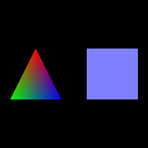
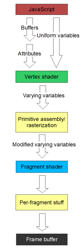
The diagram shows, in a very simplified form, how the data passed to JavaScript functions in drawScene is turned into pixels displayed in the WebGL canvas on the screen. It only shows the steps needed to explain this lesson; we’ll look at more detailed versions in future lessons.

At the highest level, the process works like this: each time you call a function like drawArrays, WebGL processes the data that you have previously given it in the form of attributes (like the buffers we used for vertices in lesson 1) and uniform variables (which we used for the projection and the model-view matrices), and passes it along to the vertex shader.

It does this by calling the vertex shader once for each vertex, each time with the attributes set up appropriately for the vertex; the uniform variables are also passed in, but as their name suggests, they don’t change from call to call. The vertex shader does stuff with this data — in lesson 1, it applied the projection and model-view matrices so that the vertices would all be in perspective and moved around according to our current model-view state — and puts its results into things called varying variables. It can output a number of varying variables; one particular one is obligatory, gl_Position, which contains the coordinates of the vertex once the shader has finished messing around with it.

Once the vertex shader is done, WebGL does the magic required to turn the 3D image from these varying variables into a 2D image, and then it calls the fragment shader once for each pixel in the image. (In some 3D graphics systems you’ll hear fragment shaders referred to as pixel shaders for that reason.) Of course, this means that it’s calling the fragment shader for those pixels that don’t have vertices in them — that is, the ones in between the pixels on which the vertices wind up. For these, it fills in points into the positions between the vertices via a process called linear interpolation — for the vertex positions that make up our triangle, this process “fills in” the space delimited by the vertices with points to make a visible triangle. The purpose of the fragment shader is to return the colour for each of these interpolated points, and it does this in a varying variable called gl_FragColor.

Once the fragment shader is done, its results are messed around with a little more by WebGL (again, we’ll get into that in a future lesson) and they are put into the frame buffer, which is ultimately what is displayed on the screen.

Hopefully, by now it’s clear that the most important trick that this lesson teaches is how to get the colour for the vertices from the JavaScript code all the way over to the fragment shader, when we don’t have direct access from one to the other.

The way we do this is to make use of the fact that we can pass a number of varying variables out of the vertex shader, not just the position, and can then retrieve them in the fragment shader. So, we pass the colour to the vertex shader, which can then put it straight into a varying variable which the fragment shader will pick up.

Conveniently, this gives us gradients of colours for free. All varying variables set by the vertex shader are linearly interpolated when generating the fragments between vertices, not just the positions. Linear interpolation of the colour between the vertices gives us smooth gradients, like those you can see in the triangle in the image above.

Let’s look at the code; we’ll work through the changes from lesson 1. Firstly, the vertex shader. It has changed quite a lot, so here’s the new code:

  attribute vec3 aVertexPosition;
  attribute vec4 aVertexColor;

  uniform mat4 uMVMatrix;
  uniform mat4 uPMatrix;

  varying vec4 vColor;

  void main(void) {
    gl_Position = uPMatrix * uMVMatrix * vec4(aVertexPosition, 1.0);
    vColor = aVertexColor;
  }

What this is saying is that we have two attributes — inputs that vary from vertex to vertex — called aVertexPosition and aVertexColor, two non-varying uniforms called uMVMatrix and uPMatrix, and one output in the form of a varying variable called vColor.

In the body of the shader, we calculate the gl_Position (which is implicitly defined as a varying variable for every vertex shader) in exactly the same way as we did in lesson 1, and all we do with the colour is pass it straight through from the input attribute to the output varying variable.

Once this has been executed for each vertex, the interpolation is done to generate the fragments, and these are passed on to the fragment shader:

  precision mediump float;

  varying vec4 vColor;

  void main(void) {
    gl_FragColor = vColor;
  }

Here, after the floating-point precision boilerplate, we take the input varying variable vColor containing the smoothly blended colour that has come out of the linear interpolation, and just return it immediately as the colour for this fragment — that is, for this pixel.

That’s all of the differences in the shaders between this lesson and the last. There are two other changes. The first is very small; in initShaders we are now getting references to two attributes rather than one; the extra lines are highlighted in red below:

  var shaderProgram;
  function initShaders() {
    var fragmentShader = getShader(gl, "shader-fs");
    var vertexShader = getShader(gl, "shader-vs");

    shaderProgram = gl.createProgram();
    gl.attachShader(shaderProgram, vertexShader);
    gl.attachShader(shaderProgram, fragmentShader);
    gl.linkProgram(shaderProgram);

    if (!gl.getProgramParameter(shaderProgram, gl.LINK_STATUS)) {
      alert("Could not initialise shaders");
    }

    gl.useProgram(shaderProgram);

    shaderProgram.vertexPositionAttribute = gl.getAttribLocation(shaderProgram, "aVertexPosition");
    gl.enableVertexAttribArray(shaderProgram.vertexPositionAttribute);

    shaderProgram.vertexColorAttribute = gl.getAttribLocation(shaderProgram, "aVertexColor");
    gl.enableVertexAttribArray(shaderProgram.vertexColorAttribute);

    shaderProgram.pMatrixUniform = gl.getUniformLocation(shaderProgram, "uPMatrix");
    shaderProgram.mvMatrixUniform = gl.getUniformLocation(shaderProgram, "uMVMatrix");
  }

This code to get the attribute locations, which we glossed over to a certain degree in the first lesson, should now be pretty clear: they are how we get a reference to the attributes that we want to pass to the vertex shader for each vertex. In lesson 1, we just got the vertex position attribute. Now, obviously enough, we get the colour attribute as well.

The remainder of the changes in this lesson are in initBuffers, which now needs to set up buffers for both the vertex positions and the vertex colours, and in drawScene, which needs to pass both of these up to WebGL.

Looking at initBuffers first, we define new global variables to hold the colour buffers for the triangle and the square:

  var triangleVertexPositionBuffer;
  var triangleVertexColorBuffer;
  var squareVertexPositionBuffer;
  var squareVertexColorBuffer;

Then, just after we’ve created the triangle’s vertex position buffer, we specify its vertex colours:

  function initBuffers() {
    triangleVertexPositionBuffer = gl.createBuffer();
    gl.bindBuffer(gl.ARRAY_BUFFER, triangleVertexPositionBuffer);
    var vertices = [
         0.0,  1.0,  0.0,
        -1.0, -1.0,  0.0,
         1.0, -1.0,  0.0
    ];
    gl.bufferData(gl.ARRAY_BUFFER, new Float32Array(vertices), gl.STATIC_DRAW);
    triangleVertexPositionBuffer.itemSize = 3;
    triangleVertexPositionBuffer.numItems = 3;

    triangleVertexColorBuffer = gl.createBuffer();
    gl.bindBuffer(gl.ARRAY_BUFFER, triangleVertexColorBuffer);
    var colors = [
        1.0, 0.0, 0.0, 1.0,
        0.0, 1.0, 0.0, 1.0,
        0.0, 0.0, 1.0, 1.0
    ];
    gl.bufferData(gl.ARRAY_BUFFER, new Float32Array(colors), gl.STATIC_DRAW);
    triangleVertexColorBuffer.itemSize = 4;
    triangleVertexColorBuffer.numItems = 3;

So, the values we provide for the the colours are in a list, one set of values for each vertex, just like the positions. However, there is one interesting difference between the two array buffers: while the vertices’ positions are specified as three numbers each, for X, Y and Z coordinates, their colours are specified as four elements each — red, green, blue and alpha. Alpha, if you’re not familiar with it, is a measure of opaqueness (0 is transparent, 1 totally opaque) and will be useful in later lessons. This change in the number of elements per item in the buffer necessitates a change to the itemSize that we associate with it.

Next, we do the the equivalent code for the square; this time, we’re using the same colour for every vertex, so we generate the values for the buffer using a loop:

    squareVertexPositionBuffer = gl.createBuffer();
    gl.bindBuffer(gl.ARRAY_BUFFER, squareVertexPositionBuffer);
    vertices = [
         1.0,  1.0,  0.0,
        -1.0,  1.0,  0.0,
         1.0, -1.0,  0.0,
        -1.0, -1.0,  0.0
    ];
    gl.bufferData(gl.ARRAY_BUFFER, new Float32Array(vertices), gl.STATIC_DRAW);
    squareVertexPositionBuffer.itemSize = 3;
    squareVertexPositionBuffer.numItems = 4;

    squareVertexColorBuffer = gl.createBuffer();
    gl.bindBuffer(gl.ARRAY_BUFFER, squareVertexColorBuffer);
    colors = []
    for (var i=0; i < 4; i++) {
      colors = colors.concat([0.5, 0.5, 1.0, 1.0]);
    }
    gl.bufferData(gl.ARRAY_BUFFER, new Float32Array(colors), gl.STATIC_DRAW);
    squareVertexColorBuffer.itemSize = 4;
    squareVertexColorBuffer.numItems = 4;

Now we have all of the data for our objects in a set of four buffers, so the next change is to make drawScene use the new data. The new code is in red again, and should be easy to understand:

  function drawScene() {
    gl.viewport(0, 0, gl.viewportWidth, gl.viewportHeight);
    gl.clear(gl.COLOR_BUFFER_BIT | gl.DEPTH_BUFFER_BIT);

    mat4.perspective(45, gl.viewportWidth / gl.viewportHeight, 0.1, 100.0, pMatrix);

    mat4.identity(mvMatrix);

    mat4.translate(mvMatrix, [-1.5, 0.0, -7.0]);
    gl.bindBuffer(gl.ARRAY_BUFFER, triangleVertexPositionBuffer);
    gl.vertexAttribPointer(shaderProgram.vertexPositionAttribute, triangleVertexPositionBuffer.itemSize, gl.FLOAT, false, 0, 0);

    gl.bindBuffer(gl.ARRAY_BUFFER, triangleVertexColorBuffer);
    gl.vertexAttribPointer(shaderProgram.vertexColorAttribute, triangleVertexColorBuffer.itemSize, gl.FLOAT, false, 0, 0);

    setMatrixUniforms();
    gl.drawArrays(gl.TRIANGLES, 0, triangleVertexPositionBuffer.numItems);

    mat4.translate(mvMatrix, [3.0, 0.0, 0.0]);
    gl.bindBuffer(gl.ARRAY_BUFFER, squareVertexPositionBuffer);
    gl.vertexAttribPointer(shaderProgram.vertexPositionAttribute, squareVertexPositionBuffer.itemSize, gl.FLOAT, false, 0, 0);

    gl.bindBuffer(gl.ARRAY_BUFFER, squareVertexColorBuffer);
    gl.vertexAttribPointer(shaderProgram.vertexColorAttribute, squareVertexColorBuffer.itemSize, gl.FLOAT, false, 0, 0);

    setMatrixUniforms();
    gl.drawArrays(gl.TRIANGLE_STRIP, 0, squareVertexPositionBuffer.numItems);
  }

And the next change… hang on, there is no next change! That was all that was necessary to add colour to our WebGL scene, and hopefully you are now also comfortable with the basics of shaders and how data is passed between them.

That’s it for this lesson — hopefully it was easier going than the first! If you have any questions, comments, or corrections, please do leave a comment below.

Next time, we’ll add code to animate the scene by rotating the triangle and the square.

<< Lesson 1Lesson 3 >>

Acknowledgments: working out exactly what was going on in the rendering pipeline was made much easier by reference to the OpenGL ES 2.0 Programming Guide, which Jim Pick recommended on his WebGL blog. As ever, I’m deeply in debt to NeHe for his OpenGL tutorial for the script for this lesson.

Welcome to my first WebGL tutorial! This first lesson is based on number 2 in the NeHe OpenGL tutorials, which are a popular way of learning 3D graphics for game development. It shows you how to draw a triangle and a square in a web page. Maybe that’s not terribly exciting in itself, but it’s a great introduction to the foundations of WebGL; if you understand how this works, the rest should be pretty simple…

Here’s what the lesson looks like when run on a browser that supports WebGL:

Click here and you’ll see the live WebGL version, if you’ve got a browser that supports it; here’s how to get one if you don’t.

More on how it all works below…

A quick warning: These lessons are targeted at people with a reasonable amount of programming knowledge, but no real experience in 3D graphics; the aim is to get you up and running, with a good understanding of what’s going on in the code, so that you can start producing your own 3D Web pages as quickly as possible. I’m writing these as I learn WebGL myself, so there may well be (and probably are) errors; use at your own risk. However, I’m fixing bugs and correcting misconceptions as I hear about them, so if you see anything broken then please let me know in the comments.

There are two ways you can get the code for this example; just “View Source” while you’re looking at the live version, or if you use GitHub, you can clone it (and future lessons) from the repository there.  Either way, once you have the code, load it up in your favourite text editor and take a look.  It’s pretty daunting at first glance, even if you’ve got a nodding acquaintance with, say, OpenGL.  Right at the start we’re defining a couple of shaders, which are generally regarded as relatively advanced… but don’t despair, it’s actually much simpler than it looks.

Like many programs, this WebGL page starts off by defining a bunch of lower-level functions which are used by the high-level code at the bottom.  In order to explain it, I’ll start at the bottom and work my way up, so if you’re following through in the code, jump down to the bottom.

You’ll see the following HTML code:

<body onload="webGLStart();">
  <a href="http://learningwebgl.com/blog/?p=28">&lt;&lt; Back to Lesson 1</a><br />

  <canvas id="lesson01-canvas" style="border: none;" width="500" height="500"></canvas>

  <br/>
  <a href="http://learningwebgl.com/blog/?p=28">&lt;&lt; Back to Lesson 1</a><br />
</body>

This is the complete body of the page — everything else is in JavaScript (though if you got the code using “View source” you’ll see some extra junk needed by my website analytics, which you can ignore). Obviously we could put more normal HTML inside the <body> tags and build our WebGL image into a normal web page, but for this simple demo we’ve just got the links back to this blog post, and the <canvas> tag, which is where the 3D graphics live.   Canvases are new for HTML5 — they’re how it supports new kinds of JavaScript-drawn elements in web pages, both 2D and (through WebGL) 3D.  We don’t specify anything more than the simple layout properties of the canvas in its tag, and instead leave all of the WebGL setup code to a JavaScript function called webGLStart, which you can see is called once the page is loaded.

Let’s scroll up to that function now and take a look at it:

  function webGLStart() {
    var canvas = document.getElementById("lesson01-canvas");
    initGL(canvas);
    initShaders();
    initBuffers();

    gl.clearColor(0.0, 0.0, 0.0, 1.0);
    gl.enable(gl.DEPTH_TEST);

    drawScene();
  }

It calls functions to initialise WebGL and the shaders that I mentioned earlier, passing into the former the canvas element on which we want to draw our 3D stuff, and then it initialises some buffers using initBuffers; buffers are things that hold the details of the the triangle and the square that we’re going to be drawing — we’ll talk more about those in a moment. Next, it does some basic WebGL setup, saying that when we clear the canvas we should make it black, and that we should do depth testing (so that things drawn behind other things should be hidden by the things in front of them). These steps are implemented by calls to methods on a gl object — we’ll see how that’s initialised later. Finally, it calls the function drawScene; this (as you’d expect from the name) draws the triangle and the square, using the buffers.

We’ll come back to initGL and initShaders later on, as they’re important in understanding how the page works, but first, let’s take a look at initBuffers and drawScene.

initBuffers first; taking it step by step:

  var triangleVertexPositionBuffer;
  var squareVertexPositionBuffer;

We declare two global variables to hold the buffers. (In any real-world WebGL page you wouldn’t have a separate global variable for each object in the scene, but we’re using them here to keep things simple, as we’re just getting started.)

Next:

  function initBuffers() {
    triangleVertexPositionBuffer = gl.createBuffer();

We create a buffer for the triangle’s vertex positions. Vertices (don’t you just love irregular plurals?) are the points in 3D space that define the shapes we’re drawing. For our triangle, we will have three of them (which we’ll set up in a minute). This buffer is actually a bit of memory on the graphics card; by putting the vertex positions on the card once in our initialisation code and then, when we come to draw the scene, essentially just telling WebGL to “draw those things I told you about earlier”, we can make our code really efficient, especially once we start animating the scene and want to draw the object tens of times every second to make it move. Of course, when it’s just three vertex positions as in this case, there’s not too much cost to pushing them up to the graphics card — but when you’re dealing with large models with tens of thousands of vertices, it can be a real advantage to do things this way. Next:

    gl.bindBuffer(gl.ARRAY_BUFFER, triangleVertexPositionBuffer);

This line tells WebGL that any following operations that act on buffers should use the one we specify. There’s always this concept of a “current array buffer”, and functions act on that rather than letting you specify which array buffer you want to work with. Odd, but I’m sure there a good performance reasons behind it…

    var vertices = [
         0.0,  1.0,  0.0,
        -1.0, -1.0,  0.0,
         1.0, -1.0,  0.0
    ];

Next, we define our vertex positions as a JavaScript list. You can see that they’re at the points of an isosceles triangle with its centre at (0, 0, 0).

    gl.bufferData(gl.ARRAY_BUFFER, new Float32Array(vertices), gl.STATIC_DRAW);

Now, we create a Float32Array object based on our JavaScript list, and tell WebGL to use it to fill the current buffer, which is of course our triangleVertexPositionBuffer. We’ll talk more about Float32Arrays in a future lesson, but for now all you need to know is that they’re a way of turning a JavaScript list into something we can pass over to WebGL for filling its buffers.

    triangleVertexPositionBuffer.itemSize = 3;
    triangleVertexPositionBuffer.numItems = 3;

The last thing we do with the buffer is to set two new properties on it. These are not something that’s built into WebGL, but they will be very useful later on. One nice thing (some would say, bad thing) about JavaScript is that an object doesn’t have to explicitly support a particular property for you to set it on it. So although the buffer object didn’t previously have itemSize and numItems properties, now it does. We’re using them to say that this 9-element buffer actually represents three separate vertex positions (numItems), each of which is made up of three numbers (itemSize).

Now we’ve completely set up the buffer for the triangle, so it’s on to the square:

    squareVertexPositionBuffer = gl.createBuffer();
    gl.bindBuffer(gl.ARRAY_BUFFER, squareVertexPositionBuffer);
    vertices = [
         1.0,  1.0,  0.0,
        -1.0,  1.0,  0.0,
         1.0, -1.0,  0.0,
        -1.0, -1.0,  0.0
    ];
    gl.bufferData(gl.ARRAY_BUFFER, new Float32Array(vertices), gl.STATIC_DRAW);
    squareVertexPositionBuffer.itemSize = 3;
    squareVertexPositionBuffer.numItems = 4;
  }

All of that should be pretty obvious — the square has four vertex positions rather than 3, and so the array is bigger and the numItems is different.

OK, so that was what we needed to do to push our two objects’ vertex positions up to the graphics card. Now let’s look at drawScene, which is where we use those buffers to actually draw the image we’re seeing. Taking it step-by-step:

  function drawScene() {
    gl.viewport(0, 0, gl.viewportWidth, gl.viewportHeight);

The first step is to tell WebGL a little bit about the size of the canvas using the viewport function; we’ll come back to why that’s important in a (much!) later lesson; for now, you just need to know that the function needs calling with the size of the canvas before you start drawing. Next, we clear the canvas in preparation for drawing on it:

    gl.clear(gl.COLOR_BUFFER_BIT | gl.DEPTH_BUFFER_BIT);

…and then:

    mat4.perspective(45, gl.viewportWidth / gl.viewportHeight, 0.1, 100.0, pMatrix);

Here we’re setting up the perspective with which we want to view the scene.  By default, WebGL will draw things that are close by the same size as things that are far away (a style of 3D known as orthographic projection).  In order to make things that are further away look smaller, we need to tell it a little about the perspective we’re using.  For this scene, we’re saying that our (vertical) field of view is 45°, we’re telling it about the width-to-height ratio of our canvas, and saying that we don’t want to see things that are closer than 0.1 units to our viewpoint, and that we don’t want to see things that are further away than 100 units.

As you can see, this perspective stuff is using a function from a module called mat4, and involves an intriguingly-named variable called pMatrix. More about these later; hopefully for now it is clear how to use them without needing to know the details.

Now that we have our perspective set up, we can move on to drawing some stuff:

    mat4.identity(mvMatrix);

The first step is to “move” to the centre of the 3D scene.  In OpenGL, when you’re drawing a scene, you tell it to draw each thing you draw at a “current” position with a “current” rotation — so, for example, you say “move 20 units forward, rotate 32 degrees, then draw the robot”, the last bit being some complex set of “move this much, rotate a bit, draw that” instructions in itself.  This is useful because you can encapsulate the “draw the robot” code in one function, and then easily move said robot around just by changing the move/rotate stuff you do before calling that function.

The current position and current rotation are both held in a matrix; as you probably learned at school, matrices can represent translations (moves from place to place), rotations, and other geometrical transformations.  For reasons I won’t go into right now, you can use a single 4×4 matrix (not 3×3) to represent any number of transformations in 3D space; you start with the identity matrix — that is, the matrix that represents a transformation that does nothing at all — then multiply it by the matrix that represents your first transformation, then by the one that represents your second transformation, and so on.   The combined matrix represents all of your transformations in one. The matrix we use to represent this current move/rotate state is called the model-view matrix, and by now you have probably worked out that the variable mvMatrix holds our model-view matrix, and the mat4.identity function that we just called sets it to the identity matrix so that we’re ready to start multiplying translations and rotations into it.  Or, in other words, it’s moved us to an origin point from which we can move to start drawing our 3D world.

Sharp-eyed readers will have noticed that at the start of this discussion of matrices I said “in OpenGL”, not “in WebGL”.  This is because WebGL doesn’t have this stuff built in to the graphics library. Instead, we use a third-party matrix library — Brandon Jones’s excellent glMatrix — plus some nifty WebGL tricks to get the same effect. More about that niftiness later.

Right, let’s move on to the code that draws the triangle on the left-hand side of our canvas.

    mat4.translate(mvMatrix, [-1.5, 0.0, -7.0]);

Having moved to the centre of our 3D space with by setting mvMatrix to the identity matrix, we start the triangle  by moving 1.5 units to the left (that is, in the negative sense along the X axis), and seven units into the scene (that is, away from the viewer; the negative sense along the Z axis).  (mat4.translate, as you might guess, means “multiply the given matrix by a translation matrix with the following parameters”.)

The next step is to actually start drawing something!

    gl.bindBuffer(gl.ARRAY_BUFFER, triangleVertexPositionBuffer);
    gl.vertexAttribPointer(shaderProgram.vertexPositionAttribute, triangleVertexPositionBuffer.itemSize, gl.FLOAT, false, 0, 0);

So, you remember that in order to use one of our buffers, we call gl.bindBuffer to specify a current buffer, and then call the code that operates on it. Here we’re selecting our triangleVertexPositionBuffer, then telling WebGL that the values in it should be used for vertex positions. I’ll explain a little more about how that works later; for now, you can see that we’re using the itemSize property we set on the buffer to tell WebGL that each item in the buffer is three numbers long.

Next, we have:

    setMatrixUniforms();

This tells WebGL to take account of our current model-view matrix (and also the projection matrix, about which more later).   This is required because all of this matrix stuff isn’t built in to WebGL.  The way to look at it is that you can do all of the moving around by changing the mvMatrix variable you want, but this all happens in JavaScript’s private space.  setMatrixUniforms, a function that’s defined further up in this file, moves it over to the graphics card.

Once this is done, WebGL has an array of numbers that it knows should be treated as vertex positions, and it knows about our matrices.   The next step tells it what to do with them:

    gl.drawArrays(gl.TRIANGLES, 0, triangleVertexPositionBuffer.numItems);

Or, put another way, “draw the array of vertices I gave you earlier as triangles, starting with item 0 in the array and going up to the numItemsth element”.

Once this is done, WebGL will have drawn our triangle.   Next step, draw the square:

    mat4.translate(mvMatrix, [3.0, 0.0, 0.0]);

We start by moving our model-view matrix three units to the right.  Remember, we’re currently already 1.5 to the left and 7 away from the screen, so this leaves us 1.5 to the right and 7 away.  Next:

    gl.bindBuffer(gl.ARRAY_BUFFER, squareVertexPositionBuffer);
    gl.vertexAttribPointer(shaderProgram.vertexPositionAttribute, squareVertexPositionBuffer.itemSize, gl.FLOAT, false, 0, 0);

So, we tell WebGL to use our square’s buffer for its vertex positions…

    setMatrixUniforms();

…we push over the model-view and projection matrices again (so that we take account of that last mvTranslate), which means that we can finally:

    gl.drawArrays(gl.TRIANGLE_STRIP, 0, squareVertexPositionBuffer.numItems);

Draw the points.  What, you may ask, is a triangle strip?  Well, it’s a strip of triangles   More usefully, it’s a strip of triangles where the first three vertices you give specify the first triangle, then the last two of those vertices plus the next one specify the next triangle, and so on.  In this case, it’s a quick-and-dirty way of specifying a square.  In more complex cases, it can be a really useful way of specifying a complex surface in terms of the triangles that approximate it.

Anyway, once that’s done, we’ve finished our drawScene function.

  }

If you’ve got this far, you’re definitely ready to start experimenting.  Copy the code to a local file, either from GitHub or directly from the live version; if you do the latter, you need index.html and glMatrix-0.9.5.min.js. Run it up locally to make sure it works, then try changing some of the vertex positions above; in particular, the scene right now is pretty flat; try changing the Z values for the square to 2, or -3, and see it get larger or smaller as it moves back and forward.  Or try changing just one or two of them, and watch it distort in perspective.  Go crazy, and don’t mind me.  I’ll wait.

…

Right, now that you’re back, let’s take a look at the support functions that made all of the code we just went over possible. As I said before, if you’re happy to ignore the details and just copy and paste the support functions that come above initBuffers in the page, you can probably get away with it and build interesting WebGL pages (albeit in black and white — colour’s the next lesson).  But none of the details are difficult to understand, and by understanding how this stuff works you’re likely to write better WebGL code later on.

Still with me?  Thanks   Let’s get the most boring of the functions out of the way first; the first one called by webGLStart, which is initGL.  It’s near the top of the web page, and here’s a copy for reference:

  var gl;
  function initGL(canvas) {
    try {
      gl = canvas.getContext("experimental-webgl");
      gl.viewportWidth = canvas.width;
      gl.viewportHeight = canvas.height;
    } catch(e) {
    }
    if (!gl) {
      alert("Could not initialise WebGL, sorry  ");
    }
  }

This is very simple.  As you may have noticed, the initBuffers and drawScene functions frequently referred to an object called gl, which clearly referred to some kind of core WebGL “thing”.  This function gets that “thing”, which is called a WebGL context, and does it by asking the canvas it is given for the context, using a standard context name.  (As you can probably guess, at some point the context name will change from “experimental-webgl” to “webgl”; I’ll update this lesson and blog about it when that happens. Subscribe to the RSS feed if you want to know about that — and, indeed, if you want at-least-weekly WebGL news.) Once we’ve got the context, we again use JavaScript’s willingness to allow us to set any property we like on any object to store on it the width and height of the canvas to which it relates; this is so that we can use it in the code that sets up the viewport and the perspective at the start of drawScene. Once that’s done, our GL context is set up.

After calling initGL, webGLStart called initShaders. This, of course, initialises the shaders (duh .  We’ll come back to that one later, because first we should take a look at our model-view matrix, and the projection matrix I also mentioned earlier.  Here’s the code:

  var mvMatrix = mat4.create();
  var pMatrix = mat4.create();

So, we define a variable called mvMatrix to hold the model-view matrix and one called pMatrix for the projection matrix, and then set them to empty (all-zero) matrices to start off with. It’s worth saying a bit more about the projection matrix here. As you will remember, we applied the glMatrix function mat4.perspective to this variable to set up our perspective, right at the start of drawScene. This was because WebGL does not directly support perspective, just like it doesn’t directly support a model-view matrix.  But just like the process of moving things around and rotating them that is encapsulated in the model-view matrix, the process of making things that are far away look proportionally smaller than things close up is the kind of thing that matrices are really good at representing.  And, as you’ve doubtless guessed by now, the projection matrix is the one that does just that.  The mat4.perspective function, with its aspect ratio and field-of-view, populated the matrix with the values that gave use the kind of perspective we wanted.

Right, now we’ve been through everything apart from the setMatrixUniforms function, which, as I said earlier, moves the model-view and projection matrices up from JavaScript to WebGL, and the scary shader-related stuff.  They’re inter-related, so let’s start with some background.

Now, what is a shader, you may ask?  Well, at some point in the history of 3D graphics they may well have been what they sound like they might be — bits of code that tell the system how to shade, or colour, parts of a scene before it is drawn.  However, over time they have grown in scope, to the extent that they can now be better defined as bits of code that can do absolutely anything they want to bits of the scene before it’s drawn.  And this is actually pretty useful, because (a) they run on the graphics card, so they do what they do really quickly and (b) the kind of transformations they can do can be really convenient even in simple examples like this.

The reason that we’re introducing shaders in what is meant to be a simple WebGL example (they’re at least “intermediate” in OpenGL tutorials) is that we use them to get the WebGL system, hopefully running on the graphics card, to apply our model-view matrix and our projection matrix to our scene without us having to move around every point and every vertex in (relatively) slow JavaScript.   This is incredibly useful, and worth the extra overhead.

So, here’s how they are set up.  As you will remember, webGLStart called initShaders, so let’s go through that step-by-step:

  var shaderProgram;
  function initShaders() {
    var fragmentShader = getShader(gl, "shader-fs");
    var vertexShader = getShader(gl, "shader-vs");

    shaderProgram = gl.createProgram();
    gl.attachShader(shaderProgram, vertexShader);
    gl.attachShader(shaderProgram, fragmentShader);
    gl.linkProgram(shaderProgram);

    if (!gl.getProgramParameter(shaderProgram, gl.LINK_STATUS)) {
      alert("Could not initialise shaders");
    }

    gl.useProgram(shaderProgram);

As you can see, it uses a function called getShader to get two things,  a “fragment shader” and a “vertex shader”, and then attaches them both to a WebGL thing called a “program”.  A program is a bit of code that lives on the WebGL side of the system; you can look at it as a way of specifying something that can run on the graphics card.  As you would expect, you can associate with it a number of shaders, each of which you can see as a snippet of code within that program; specifically, each program can hold one fragment and one vertex shader. We’ll look at them shortly.

    shaderProgram.vertexPositionAttribute = gl.getAttribLocation(shaderProgram, "aVertexPosition");
    gl.enableVertexAttribArray(shaderProgram.vertexPositionAttribute);

Once the function has set up the program and attached the shaders, it gets a reference to an “attribute”, which it stores in a new field on the program object called vertexPositionAttribute. Once again we’re taking advantage of JavaScript’s willingness to set any field on any object; program objects don’t have a vertexPositionAttribute field by default, but it’s convenient for us to keep the two values together, so we just make the attribute a new field of the program.

So, what’s the vertexPositionAttribute for? As you may remember, we used it in drawScene; if you look now back at the code that set the triangle’s vertex positions from the appropriate buffer, you’ll see that the stuff we did associated the buffer with that attribute. You’ll see what that means in a moment; for now, let’s just note that we also use gl.enableVertexAttribArray to tell WebGL that we will want to provide values for the attribute using an array.

    shaderProgram.pMatrixUniform = gl.getUniformLocation(shaderProgram, "uPMatrix");
    shaderProgram.mvMatrixUniform = gl.getUniformLocation(shaderProgram, "uMVMatrix");
  }

The last thing initShaders does is get two more values from the program, the locations of two things called uniform variables. We’ll encounter them soon; for now, you should just note that like the attribute, we store them on the program object for convenience.

Now, let’s take a look at getShader:

  function getShader(gl, id) {
      var shaderScript = document.getElementById(id);
      if (!shaderScript) {
          return null;
      }

      var str = "";
      var k = shaderScript.firstChild;
      while (k) {
          if (k.nodeType == 3)
              str += k.textContent;
          k = k.nextSibling;
      }

      var shader;
      if (shaderScript.type == "x-shader/x-fragment") {
          shader = gl.createShader(gl.FRAGMENT_SHADER);
      } else if (shaderScript.type == "x-shader/x-vertex") {
          shader = gl.createShader(gl.VERTEX_SHADER);
      } else {
          return null;
      }

      gl.shaderSource(shader, str);
      gl.compileShader(shader);

      if (!gl.getShaderParameter(shader, gl.COMPILE_STATUS)) {
          alert(gl.getShaderInfoLog(shader));
          return null;
      }

      return shader;
  }

This is another one of those functions that is much simpler than it looks.  All we’re doing here is looking for an element in our HTML page that has an ID that matches a parameter passed in, pulling out its contents, creating either a fragment or a vertex shader based on its type (more about the difference between those in a future lesson) and then passing it off to WebGL to be compiled into a form that can run on the graphics card.  The code then handles any errors, and it’s done! Of course, we could just define shaders as strings within our JavaScript code and not mess around with extracting them from the HTML — but by doing it this way, we make them much easier to read, because they are defined as scripts in the web page, just as if they were JavaScript themselves.

Having seen this, we should take a look at the shaders’ code: 

<script id="shader-fs" type="x-shader/x-fragment">
  precision mediump float;

  void main(void) {
    gl_FragColor = vec4(1.0, 1.0, 1.0, 1.0);
  }
</script>

<script id="shader-vs" type="x-shader/x-vertex">
  attribute vec3 aVertexPosition;

  uniform mat4 uMVMatrix;
  uniform mat4 uPMatrix;

  void main(void) {
    gl_Position = uPMatrix * uMVMatrix * vec4(aVertexPosition, 1.0);
  }
</script>

The first thing to remember about these is that they are not written in JavaScript, even though the ancestry of the language is clearly similar.  In fact, they’re written in a special shader language — called GLSL — that owes a lot to C (as, of course, does JavaScript). 

The first of the two, the fragment shader, does pretty much nothing; it has a bit of obligatory boilerplate code to tell the graphics card how precise we want it to be with floating-point numbers (medium precision is good because it’s required to be supported by all WebGL devices — highp for high precision doesn’t work on all mobile devices), then simply specifies that everything that is drawn will be drawn in white.  (How to do stuff in colour is the subject of the next lesson.)

The second shader is a little more interesting.   It’s a vertex shader — which, you’ll remember, means that it’s a bit of graphics-card code that can do pretty much anything it wants with a vertex.  Associated with it, it has two uniform variables called uMVMatrix and uPMatrix.  Uniform variables are useful because they can be accessed from outside the shader — indeed, from outside its containing program, as you can probably remember from when we extracted their location in initShaders, and from the code we’ll look at next, where (as I’m sure you’ve realised) we set them to the values of the model-view and the projection matrices.  You might want to think of the shader’s program as an object (in the object-oriented sense) and the uniform variables as fields. 

Now, the shader is called for every vertex, and the vertex is passed in to the shader code as aVertexPosition, thanks to the use of the vertexPositionAttribute in the drawScene, when we associated the attribute with the buffer.  The tiny bit of code in the shader’s main routine just multiplies the vertex’s position by the model-view and the projection matrices, and pushes out the result as the final position of the vertex.

So, webGLStart called initShaders, which used getShader to load the fragment and the vertex shaders from scripts in the web page, so that they could be compiled and passed over to WebGL and used later when rendering our 3D scene.

After all that, the only remaining unexplained code is setMatrixUniforms, which is easy to understand once you know everything above

  function setMatrixUniforms() {
    gl.uniformMatrix4fv(shaderProgram.pMatrixUniform, false, pMatrix);
    gl.uniformMatrix4fv(shaderProgram.mvMatrixUniform, false, mvMatrix);
  }

So, using the references to the uniforms that represent our projection matrix and our model-view matrix that we got back in initShaders, we send WebGL the values from our JavaScript-style matrices.

Phew!  That was quite a lot for a first lesson, but hopefully now you (and I) understand all of the groundwork we’re going to need to start building something more interesting — colourful, moving, properly three-dimensional WebGL models. To find out more, read on for lesson 2.

<< Lesson 0Lesson 2 >>

Acknowledgments: obviously I’m deeply in debt to NeHe for his OpenGL tutorial for the script for this lesson, but I’d also like to thank Benjamin DeLillo and Vladimir Vukićević for their WebGL sample code, which I’ve investigated, analysed, probably completely misunderstood, and eventually munged together into the code on which I based this post . Thanks also to Brandon Jones for glMatrix. Finally, thanks to James Coglan, who wrote the general-purpose Sylvester matrix library; the first versions of this lesson used it instead of the much more WebGL-centric glMatrix, so the current version would never have existed without it.